- DOI 10.31509/2658-607x-202264-135
MODELING THE DYNAMICS OF FOREST ECOSYSTEMS TAKING INTO ACCOUNT THEIR STRUCTURAL HETEROGENEITY AT DIFFERENT FUNCTIONAL AND SPATIAL LEVELS
![]()
Original Russian Text © 2022 V. N. Shanin, P. V. Frolov, I. V. Priputina, O. G. Chertov, S. S. Bykhovets, E. V. Zubkova, A. M. Portnov, G. G. Frolova, M. N. Stamenov, P. Y. Grabarnik published in Forest Science Issues Vol. 5, No 3, Article 112.
V. N. Shanin1, 2, P. V. Frolov1, I. V. Priputina1, O. G. Chertov3, S. S. Bykhovets1, E. V. Zubkova1, A. M. Portnov1, G. G. Frolova1, M. N. Stamenov1, P. Y. Grabarnik1
1Institute of Physicochemical and Biological Problems in Soil Science
Pushchino Scientific Center for Biological Research of the Russian Academy of Sciences, Institutskaya 2, 142290 Pushchino, Russia
2Center for Forest Ecology and Productivity of the Russian Academy of Sciences
Profsoyuznaya st., 84/32, bld. 14, 117997 Moscow, Russia
3Bingen University of Applied Sciences
Berlin Str. 109, 55411 Bingen, Germany
E‑mail: shaninvn@gmail.com
Received: 08.09.2022
Revised: 15.10.2022
Accepted: 28.10.2022
Many problems of modern forest ecology require analysis of the conjugated dynamics of processes occurring at different spatio-temporal scales of the functioning of plant communities and soils resulted from their interaction under the influence of all edaphic and anthropogenic factors. Mathematical models can be an effective tool for such analysis. The aim of this study is to present the implementation of new model system that makes it possible to reproduce in simulation experiments the spatial structure of forest phytocenoses formed by tree and grass-shrub layers, as well as associated heterogeneity of soil conditions and the diversity of ecological niches at different hierarchical levels. To determine the required level of detail of the spatial heterogeneity of forest biogeocenoses related to the processes of their multi-scale functioning, experimental studies were carried out on permanent sampling plots in the Prioksko-Terrasny State Natural Biosphere Reserve and in the “Kaluzhskie Zaseki” State Nature Reserve. The spatial structure of communities and related heterogeneity of ecological conditions were studied using traditional soil and geobotanical, as well as modern instrumental methods. The obtained data were used to construct the algorithms and to estimate the parameters of different blocks of the new system of models. The implementation of a spatially-explicit process-based system of models has shown its ability to reproduce the dynamics of forest ecosystems, taking into account the species composition and spatial structure of different layers of vegetation and the associated patchiness of soil conditions. Due to a wide range of interrelated ecosystem characteristics implemented in the system of models it is possible to simulate productivity, biological turnover of C and N, and the dynamics of forest ecosystems, taking into account their typical spatial structure at different scales. This improves understanding of ecosystem processes and their contribution to maintaining the sustainable functioning of forests, which can be used for predictive assessments of the efficiency of forest management techniques and in solving other forestry and environmental problems.
Key words: simulation models, spatial structure, tree stand productivity, ground layer vegetation, forest soils, soil nutrients, carbon cycle.
INTRODUCTION
Conservation of biodiversity and biosphere functions of the Earth’s forest cover is impossible without identifying mechanisms for sustainable maintenance of the structure and functioning of forest ecosystems. In the case of old-growth forests, they are characterized by multispecies and, as a rule, multilayer and uneven-aged composition, as well as with high spatial heterogeneity of the soil cover. The necessary change of generations is ensured in them, including those determining the successional dynamics of ecosystems.
An integral characteristic of all terrestrial ecosystems is their spatial structure (Eastern European Forests …, 2004; Karpachevsky, 1981). It is manifested, for example, in the horizontal and vertical arrangement of plants in the biogeocenosis and the vertical structure of the canopy. In addition, spatial structure determines many soil processes. The interest in analyzing the spatial structure of communities and its changes is due to the assumption that this analysis can help in the study of ecological processes occurring in the community. It is generally accepted that the spatial structure of communities is an indicator of habitat diversity and full utilization of environmental resources by plants. It is the mutual spatial arrangement of individuals that largely determines such important biological processes in plant communities as successful species renewal and competition for resources (Kolobov et al., 2015; Kolobov, Frisman, 2018). Equally relevant are the issues related to the analysis of mechanisms of formation of feedbacks between the functioning of biota and its habitat (in particular, soil cover), which manifest themselves at different hierarchical levels and with different characteristic times. The joint effect of different ecological processes can be multidirectional (reducing the resulting effect) or co-directional (accelerating time and/or increasing the intensity of its manifestation), and, in addition, can have specific features at different spatial scales. Nevertheless, it is often possible to show that the observed complexity of processes can result from the composition of simple interactions between individuals, primarily determined by the spatial structure, which, in turn, is formed under these processes.
The problem of joint analysis of structure and scale is one of the most important problems of ecology, which unites population biology and the science of environmental conditions (edaphology) and relates basic and applied ecology (Levin, 1992). A large number of topical issues, such as predicting the ecological consequences of global climate change, preserving biodiversity and ecosystem stability, require the study of phenomena occurring at a wide range of scales of space, time and levels of ecological organization, as it is impossible to identify a particular scale to describe the entire variety of natural phenomena. Accordingly, the analysis of spatial relationships of biota components should be carried out at different spatial scales as from the microlevel, defined by the functioning of microbocenosis in soil loci, to the level of an individual (tree or grass-shrub plant) interacting with its nearest neighbors, and further to the relationships of plant populations of ground cover and forest stands, i.e. at the level of biocenosis.
In recent years, the analysis of the spatial structure and spatial heterogeneity of ecosystems, and their biotic components has acquired a qualitatively new theoretical and practical level. This is largely due to the accelerated development of modern technologies of ground and airborne 3D laser scanning, as well as aerial photography with the use of drones. The possibility of obtaining such sets of measurements, along with the use of methods of mathematical processing of spatially distributed data, makes it possible to use previously unavailable approaches to the analysis of the structure of ecosystems at different spatial levels and to obtain fundamentally new information on the mechanisms of internal organization, functioning and sustainable development of biogeocenoses. Despite advances in spatial data analysis, questions that can be answered using spatial statistical techniques remain within the scope of identifying the features of the structures formed. It means that it became possible to calculate the probability that the observed structure is related to spatially related phenomena or processes. However, spatial statistical methods do not allow us to explain the mechanisms of particular structure formation and what ecological processes may cause the observed patterns. An approach is needed that combines spatial statistical methods and individual-based simulation models that reproduce the functioning and quantitative characteristics of ecosystems based on mathematical or mechanistic descriptions of processes.
The role of the forest ecosystems living ground cover is rarely considered when analyzing the carbon balance of areas (Goulden et al., 1997; Law et al., 1999). However, in many widespread types of boreal forests, tree canopy density is low, which ensures high availability of solar radiation for plants of the grass and shrub layer and, as a consequence, determines high photosynthesis intensity (Baldocchi et al., 2000). No less important is the influence of the grass-shrub layer on the regeneration of woody plants.
Vegetation litter in forest ecosystems plays the role of a nutrient source, and the ratio of its input and decomposition rates regulates the rate of nutrient dynamics in the soil and, consequently, the production process (Nilsson, Wardle, 2005; Kolari et al., 2006). Hence, changes in the structure of plant communities lead to qualitative and quantitative changes in forest litter, which, in turn, has a direct impact on soil carbon accumulation (Karpachevsky, 1981; Chertov, 1981; Hättenschwiler, Gasser, 2005). In addition, the nature of vegetation litter and forest cover formed by it determine in many respects the structure of soil microbocenosis in charge of transformation and mineralization processes of organic matter and nitrogen compounds in soils.
The structural complexity analysis of forest ecosystems reveals the mechanisms and processes that determine their non-linear dynamics and lead to the formation of specific spatial organization of forest vegetation. An indispensable tool for such an analysis is simulation modeling, which allows to formalize a quantitative description of the dynamics of forest ecosystem elements, spatial relationships between elements and the role of interactions between components in maintaining its sustainability. Forest ecosystem stability in this case is understood as its ability to maintain structure, functioning, dynamics and productivity in the process of development, both in the absence of external disturbances and under various kinds of impacts. Simulation experiments will improve understanding of the complex interactions between different ecosystem components and the processes that determine the structure, stability and productivity of complex plant communities.
For domestic forest ecology, the relevance of the development of mathematical models as a tool for predicting productivity and assessing ecosystem functions of forests is determined by the transition of the country’s forest sector to an intensive model of development. Such model is focused on shorter timeframes for obtaining marketable products, including through the wider introduction of planted forest crops and forest plantations in the practice of forest management (Romanov et al., 2016). Apart from the issues of economic feasibility of expenditures on artificial reforestation and afforestation in different soil and climatic conditions, the issue of substantiation of optimal forestry scenarios that ensure high timber production while preserving ecological functions of forests becomes no less important.
Simulation models of forest ecosystems usually consist of the following blocks: models of tree regeneration and die-off, models of tree biomass production, models of competition, and models of soil organic matter dynamics. They can also include models of living ground cover, tools to simulate forest management activities (planting and maintenance of forest crops, felling, etc.) and various types of disturbances (fires, windfall, phytopathogens). We have given more detailed reviews of models of different types previously (Grabarnik et al., 2019b; Chertov et al., 2019).
Renewal models. One of the most important tasks in analyzing the dynamics of forest ecosystems is the study of regeneration processes. Its solution allows us to get closer to understanding the basics of sustainable development of ecosystems. One of the generally accepted concepts of forest cenosis dynamics is the “gap” model (Korotkov, 1991; McCarthy, 2001). In this case, the forest cover is represented as a “patchiness” of small areas occupied by cohorts of trees at different stages of development and formed on the site of fallen trees of previous generations. Here, the emergence of regrowth and its development to the adult tree stage is related to the falling off of trees and the location of neighboring large trees that form the spatial “frame” of the ecosystem. Empirical models describe the dependence of density and species composition of forest regeneration on geographic and climatic factors (Pukkala, Kolström, 1992), as well as habitat characteristics and species composition of the upper forest stand (Pukkala et al., 2012). Tree establishment in renewal models considers tree establishment at the local level depending on the presence of nearest neighbors (Kuuluvainen et al., 1993; Fajardo et al., 2006; Wiegand et al., 2009; Pommerening, Grabarnik, 2019). Dynamic spatial point process models account for competition between upper layer trees to answer fundamental questions related to stand dynamics and explain the emergence of spatial structures (Moeur, 1997).
Competition models. Competition in individual-based models is described with varying degrees of spatial detail. In general, there are several main approaches. In the most general case, competition indices (Daniels et al., 1986) are used to summarize the strength and direction of interactions between plants in a community. A development of this approach is the application of ecological field theory in individual-based models to describe competitive interactions (Zhukova, 2012; Seidl et al., 2012). In a number of models, the two main types of competition (for light and for soil resources) are considered separately (or only one of them is considered). When modeling crown competition, both simple models that consider the overlap of so-called “shading zones” (actually vertical projections of crowns) of neighboring trees and more complex models that use three-dimensional representation of crowns (in discrete models crowns are usually approximated by square prisms) and precise calculation of sunlight passing through the canopy are used (Brunner, 1998; Martens et al, 2000; Stadt, Lieffers, 2000; Olchev et al., 2009; Lebedev, Chumachenko, 2011). In particular cases, crowns can be represented as flat “screens” (Korzukhin, Ter‑Mikaelian, 1995), or more generally the model is able to account for the internal structure of the crown (heterogeneity in biomass distribution), such as the Mixfor‑3D model (Olchev et al., 2009). More complex models reproduce the spatial structure of the crown with high accuracy (Renshaw, 1985). Among such models, the LIGNUM model (Perttunen, 2009), which is based on L‑systems and reproduces the crown architecture in detail, is also noteworthy. The LIGNUM model is designed to simulate processes at the individual tree level, but attempts have been made to model the growth of single-species forest stands (Sievänen et al., 2008). The PICUS model (Lexer, Hönninger, 2001) is an individual-based three-dimensional gap-model that allows the heterogeneity of the forest canopy to be taken into account when calculating illuminance using a three-dimensional ray path model and terrain features. The spatially-explicit FORRUS‑S model (Chumachenko et al., 2003) belongs to the class of bioecological models that simulate the processes of birth, growth and death of individuals. The model considers the influence of habitat conditions and light regime on forest stand growth and allows simulating different regimes of multipurpose forest management, which makes it an important element of forest management planning in forest areas. In recent years, an approach that simplifies the vertical structure of a stand into several “layers” corresponding to different stand layers has become popular (e.g., Kolobov, 2013; Collalti et al., 2014).
Several regression models describing the dependence of root mass on depth have been proposed to describe the spatial structure of root systems (Strong, LaRoi, 1985; Gale, Grigal, 1987; Starr et al., 2009, 2012). It should be noted that models of root systems are usually not independent, but are part of more complex models of natural or agroecosystems. It should be especially emphasized that even many modern simulation models do not have a block simulating competition for water and mineral nutrition elements (only competition for light is simulated or generalized competition indices are used). In the simplest models of root competition, soil nutrients are equally distributed among all plants in the simulated area, and the uptake rates of water and mineral nutrition elements decrease with distance from the trunk (Yastrebov, 1996; Casper et al., 2003). Many of the approaches mentioned above are attempts to “tie” the intensity of underground competition to the intensity of aboveground competition (much more easily defined). There is also a whole group of ecosystem models that consider limiting stand productivity by the amount of N available in soil, such as iLand (Seidl et al., 2012), PICUS (Lexer, Hönninger, 2001), 4C (Lasch‑Born et al., 2020), and TRIPLEX (Zhou et al., 2008), but in which soil is treated as a common resource that is spatially homogeneous and biomass growth limited by the amount of N available is calculated using species-specific response functions. Nevertheless, a number of studies have unambiguously shown that the content of available nutrients and organic matter in soils can differ by more than an order of magnitude at distances of only tens of centimeters (Kuzyakova et al., 1997; Spielvogel et al., 2009).
In simulation models that operate objects on a regular lattice, the concept of a “nutrition zone” is introduced, i.e., the area (group of cells) occupied by the roots of a particular tree. Typically, in such models, root mass is assumed to be uniformly distributed over the entire nutrition area of a particular tree (Goreaud et al., 2002; Raynaud, Leadley, 2005). It should also be noted here that few models of this kind have been developed to simulate the dynamics of multi-species stands and thus account for species-specific differences in root distribution (Mao et al., 2015; Shanin et al., 2015a). The EFIMOD model system (Komarov et al., 2003a) uses a relatively simplified representation of the processes of competition for light and mineral nitrogen in soil and biomass production. The EFIMOD model system (Komarov et al., 2003a) takes into account the influence of only the above two factors on productivity. The model is based on the assumption that all possible uncertainties will be leveled out when calculating the average dynamics in a population of interacting individuals (Komarov, 2010).
In stands formed by several tree species with different ecological and cenotic strategies, spatial heterogeneity in resource availability can be much higher than in monocultures (Grime, 2002; Pretzsch, 2014). This is the most likely reason for the higher productivity of multi-species stands compared to single-species stands (Bielak et al., 2014; Cavard et al., 2011; Pretzsch et al., 2015), as confirmed both by experimental studies and simulation modeling (Rötzer, 2013; Moghaddam, 2014; Toïgo et al., 2015; Forrester, Bauhus, 2016; Pretzsch, Schütze, 2021). Accordingly, competition models should take into account species-specific features of crown development and root systems of trees.
Cellular-automata models of plant populations. In models of this type, the main object of the model is an individual, which changes its state and characteristics in time according to some rules. They include dependence on the state and/or size of neighboring objects (Komarov, 1982; Berger et al., 2008; Herben, Widova, 2012; Oborny et al., 2012, etc.). This approach is used to analyze the joint dynamics of a set of discrete objects having spatial coordinates. General properties of the modeled system are controlled and determined through local interactions between the objects composing the system. This property allows building meaningful models of complex multicomponent systems, such as, for example, a multispecies community of plants characterized by different ecological and biological properties. At the same time, these models exhibit nonlinear properties meaning that spatio-temporal models with simple developmental rules for individuals can reproduce complex patterns of population dynamics. Using cellular-automata models, for example, the effects of competition and seed dispersal on the resilience of plant communities under severe disturbances have been studied (Komarov, 1982; Matsinos, Troumbis, 2002; Komarov et al., 2003b). Cellular automata have also been used to describe invasion processes of species with different abilities to compete for space compared to local community species (Arii, Parrott, 2006). Combining the techniques of cellular automata, L‑systems and matrix modeling (Frolov et al., 2015, 2020a, 2020b) allows us to predict the population dynamics of multispecies communities taking into account species-specific features of growth, development, and response to environmental factors, and improves the accuracy of the mass-balance approach to predicting their productivity.
Soil organic matter dynamic models. In early forest ecosystem models, blocks for simulating soil organic matter dynamics were either absent or presented in the form of unchanging edaphic conditions (Shugart et al., 1992). Active development of soil organic matter dynamics models reached its peak at the end of the XX century. Models of this period are often integrated into models of biogeochemical element cycles. Among foreign models, the CENTURY model is the best known (Parton et al., 1988), and among domestic models, the ROMUL and Romul_Hum models analyzed below (Chertov et al., 2001; Chertov et al., 2017a, 2017b; Komarov et al., 2017a). The VSD+ (Posch, Reinds, 2009) and SMARTml (Bonten et al., 2011) models allow modeling the dynamics of a small number of soil parameters and are used to simulate the response of terrestrial ecosystems, including forests, to the input of acid-forming and eutrophying compounds with precipitation. The ForSAFE forest soil chemical dynamics model (Sverdrup et al., 2007) can be combined with the VEG ground cover vegetation model (Belyazid et al., 2011). Another group of researchers from the UK continues to develop the MAGIC model (Cosby et al., 2001; Oulehle et al., 2012), which allows modeling changes in soil acid-alkaline properties and the in-soil nitrogen cycle.
According to the nature of the use of soil organic matter models in the structure of forest ecosystem models, they can be divided into two groups. The first group includes model systems without “feedback”, i.e. those that do not take into account the impact of soil changes on forest vegetation productivity. Examples of such models are forestry models of economic productivity with conversion of taxation parameters to carbon and forest residue pools through conversion functions, such as in the EFISCEN (Nabuurs et al., 2000) and MELA (Hirvelä et al., 2017) models. In feedback model systems, soil models are functionally embedded in the structure of ecosystem process models (Parton et al., 1988; Chertov et al., 1999; Komarov et al., 2003a; Grabarnik et al., 2019a). The main driver of the feedback is soil nitrogen available to plants, produced by mineralization of soil organic matter. In turn, the role of N in plant productivity in process models is accounted for either as an external factor (just like temperature and humidity) by correction factors to the underlying growth function (Kellomäki et al., 1993; Seidl et al., 2012) or as a resource used to synthesize plant biomass (Komarov et al., 2003a; Shanin et al., 2019), for which biomass growth is calculated. At the same time, the change in soil organic matter reserves under the influence of plant fall directly affects the production of available nitrogen.
The following problems can be formulated within the framework of analysis by means of simulation modeling of the relationship between the structure of forest communities and their sustainable functioning:
- Mathematical description of the structure of complex plant communities based on modern methods of spatial statistics. The solution of this problem will make it possible to model the features of spatial structure necessary for inclusion in more complex models of self-organization of vegetation cover of forest ecosystems.
- Construction of individual-based spatially-explicit simulation models of forest ecosystem dynamics. These models should reproduce (a) the mechanisms of competitive relationships for light and soil resources, which are determined by the spatial structure of phytocenoses, which will allow to obtain in simulation experiments realistic reconstructions of structural changes in forest ecosystems; (b) the dynamics of growth of individual plants depending on the amount of obtained resources and habitat conditions. An important property of competition models should be the ability to imitate plant adaptation to heterogeneous environmental conditions and competitive pressure from neighboring plants.
- Finding the required level of detail in the description of endo- and exogenous processes occurring in forest ecosystems, which is required to ensure scalability of the model system.
- Development of methods for modeling structural and functional organization, population dynamics and productivity of living ground cover plants. The solution of this problem will improve the description of biophilic elements turnover taking into account the production of phytomass of ground cover plants and spatial variation of soil organic matter dynamics as a consequence of heterogeneity of living ground cover structure. This problem is closely related to the problem of developing a model of natural regeneration of trees, taking into account the spatial structure of the stand and ground cover and the ecotope conditions formed by them.
- Development of soil organic matter dynamics models (mineralization and humification processes) taking into account spatial heterogeneity in plant litter input and soil hydrothermal regime. The latter will require the development of a spatially-explicit model of soil climate, taking into account the following factors of its formation: the heterogeneity of vegetation and soil cover structure, including the influence of vegetation and microrelief.
EXPERIMENTAL STUDIES
According to existing concepts, the spatial structure of forest ecosystems changes hierarchically, reflecting the total effects of different factors and multiple processes underlying spatial patterns at one or another scale (Kuuluvainen et al., 1998; Kulha et al., 2018; Tikhonova, Tikhonov, 2021). Meanwhile, some factors and processes form patterns at multiple scales (Elkie, Rempel, 2001). To determine the required level of detail of the spatial heterogeneity of forest biogeocenoses associated with the processes of their functioning at different scales, we conducted a set of experimental field studies. The results of them were used to modify and parameterize new version of the model system.
Studies were carried out at the following two key sites — the Prioksko-Terrasny State Natural Biosphere Reserve (south of Moscow Region, coniferous-broadleaved forest subzone) and “Kaluzhskie Zaseki” State Nature Reserve (south-east of Kaluga Region, broadleaved forest subzone). The choice of forest communities with participation or dominance of broad-leaved species as objects of study is not accidental. In the Russian studies, there are quite a few publications related to the study of the biogenic cycle and functioning conditions of taiga forests (Kazimirov, Morozova, 1973; Lukina, 1996; Bobkova et al., 2000; Nikonov et al., 2002; Native …, 2006; Lukina et al., 2019). Data from these and other publications were used in the development of the first versions of the EFIMOD model system (Komarov et al., 2003a) and its subsequent modifications, which showed good reproduction in simulation estimates of the features of biogenic carbon cycling in different types of spruce, pine and small-leaved forests (Chertov et al., 2015; Komarov, Shanin, 2012). Expanding the scope of EFIMOD application by including parameters for broad-leaved species in stand submodels required not only quantitative data on their competition for resources, growth parameters, and biomass distribution among organs, and conditions for successful regeneration, but also a special analysis of the peculiarities of formation and dynamics of the spatial structure of such stands.
When planning field studies at key sites, we proceeded from the understanding that the mutual arrangement of trees of different species and sizes determines not only the competition between them for light and soil nutrition elements, but also forms the variability of ecological conditions under the forest canopy. It, in turn, provides a variety of ecological niches of different scales. It is important for maintaining the productivity and ecosystem functions of forests, their biodiversity and sustainable development. Accordingly, when conducting field studies, we focused, on the one hand, on the layer-component structure of forest biogeocenoses (stand, regrowth, ground cover, forest litter, root-inhabitable soil horizons) and, on the other hand, on different scale levels of their manifestation and functioning (community, cenopopulation, individual plants, plant organs).
Brief characterization of the study objects
A 1 ha (100 × 100 m) permanent sample plot in the Prioksko-Terrasny State Natural Biosphere Reserve was laid out in 2016. The sides of the permanent sample plots are oriented along the magnetic meridian; additionally, the area is divided into 20 × 20 m squares, the corners and centers of which are marked with milestones. In mixed uneven-aged stands Betula spp., Picea abies L. and Pinus sylvestris L. predominate, and Populus tremula L. occurs less frequently. The second layer is represented mainly by Tilia cordata Mill. and Picea abies, with Quercus robur L. occurring less frequently. The average age of trees in the first layer varies from 70–75 years (Tilia cordata, Picea abies) to 110–115 years (Quercus robur, Pinus sylvestris). The spatial arrangement of trees of different species within the sample plot is shown in Fig. 1. The sparse stand character in the south-western part of the permanent sample plot is associated with mass mortality of generative trees of Picea abies as a result of bark beetle (Ips typographus (Linnaeus, 1758)) damage in 2012. Picea abies and Tilia cordata predominate in regrowth. Vaccinium myrtillus L., Pteridium aquilinum (L.) Kuhn, Calamagrostis arundinacea Roth and Convallaria majalis L. dominate in different sections of the permanent sample plot in the grass-shrub layer. The soil cover is classified as sod-podbur (Classification …, 2004) or Albic Luvisol (WRB, 2015). More detailed characterization of the soil and vegetation conditions of the permanent sample plot is reflected in publications of Shanin et al. (2018) and Priputina et al. (2020).
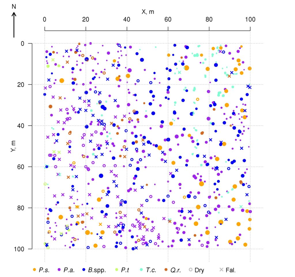
Figure 1. Plan-scheme of the stand at the permanent sample plot of the Prioksko-Terrasny Reserve P.s. — Pinus sylvestris, P.a. — Picea abies, B.spp. — Betula spp., P.t. — Populus tremula, T.c. — Tilia cordata, Q.r. — Quercus robur, Dry — dead standing trees, Fal. — fallen trees since the initial accounting in 2016
Field studies at the permanent sample plot of the Prioksko-Terrasny Reserve included thematic blocks in accordance with the component structure of biogeocenoses. Studies of the tree layer included the following:
- Mapping of the stand, determination of ontogenetic states and Kraft classes (for living trees), heights, trunk diameters at breast height (DBH) and tree coordinates using a Laser Technology TruPulse 360B laser rangefinder with height and magnetic azimuth functions, which allowed us to prepare the scenario required for validation of the model system.
- Multiseasonal aerial survey of forest stands using quadrocopters to create orthophotos of the permanent sample plot in the Prioksko-Terrasny Reserve. DJI Phantom 4 and Phantom 4 Pro quadcopters were used. The flights were performed in automatic mode according to mosaic flight mode shooting scenario with 80–95% image overlap.
- Measuring tree crown projections by visual interpretation of orthophotos derived from the processing of aerial photographs. Steps 2 and 3 are necessary to parameterize the procedure describing the relationship between the dimensional characteristics of the trunk and crown of the tree.
- Regrowth demographic survey at 5 survey plots (20 × 20 m).
- Analysis of distribution in space of needle/leaf and other fractions of aboveground litterfall of 6 tree species (Picea abies, Pinus sylvestris, Betula spp., Quercus robur, Tilia cordata, Acer platanoides) using a series of litter traps installed at different distances from the trees taking into account their size characteristics. Based on the data obtained, the species-specific spatial distribution function of needle/leaf litter was parameterized.
Studies of the grass-shrub layer included the following:
- Multiscale spatial mapping of dominant species, estimation of projective cover of different species taking into account the density of tree canopy in the places of their growth.
- Determination of heterogeneity of growing conditions of plant cenopopulations within the sample area: illumination (available photosynthetically active radiation (PAR)) and soil moisture were measured instrumentally, sub-horizons (L, F, H) of litter and humus-accumulative soil horizon were sampled to determine C and N content. These data allowed validation of the model system in terms of the confinement of the spatial structure of living ground cover to local ecological conditions.
- Determination of light conditions under the stand canopy for different variants of projective cover and ranges of tolerance of dominant species to light and soil moisture factors.
- Controlled experiment to determine the dependence of photosynthesis intensity of Pteridium aquilinum, Calamagrostis arundinacea and Convallaria majalis on soil moisture. The experimental data obtained in steps 3 and 4 were used for parameterization of species-specific photosynthesis parameters and productivity response functions of the studied species to the moisture content of the root habitable soil layer.
- Sampling of dominant species to obtain data on biomass, carbon and nitrogen content in different organs of living plants and plant litter. Based on these data, the coefficients of the rank distribution function were calculated, which are needed to calculate the production characteristics of the living ground cover submodel.
Soil studies included the following:
- Study of the spatial distribution of organic matter characteristics (Corg, Ntotal, C:N) of forest litter and organomineral horizons of soils depending on the location of trees of different species, crown density and species composition of the grass-shrub layer.
- All-year monitoring of temperature and moisture of litter and organomineral soil horizons, as well as the amount of atmospheric precipitation entering the canopy of the stand depending on its density and species composition. Experimental data obtained from steps 1 and 2 were used for validation of submodels of hydrothermal regime and soil organic matter dynamics.
The permanent sample plot in the “Kaluzhskie Zaseki” State Nature Reserve is located in an old-growth polydominant broadleaved forest without signs of logging and other disturbances in the Southern section of the Reserve and covers an area of 10.8 ha (200 × 540 m). The sample plot was established in 1986–1988 under the direction of Prof. O. V. Smirnova. A re-census was conducted in 2016–2018, and a second stand mapping on a 40 × 40 m plot was conducted in 2021. The tree stand has a layered structure and consists mainly of Quercus robur, Fraxinus excelsior L., Tilia cordata, Acer platanoides, Acer campestre L., Ulmus glabra Huds., Betula spp. and Populus tremula. The diversity of species composition of the tree stand upper layer can be seen from an aerial photograph taken in the fall (Fig. 2). Some Quercus robur individuals are over 300 years old, and the maximum age of trees of other species exceeds 150 years (Shashkov et al., 2022). The undegrowth is formed by Corylus avellana L., Euonymus europaeus L., E. verrucosus Scop., Lonicera xylosteum L., Prunus padus L.; and Tilia cordata, Ulmus glabra, Acer platanoides and Acer campestre are mainly represented in the regrowth. The ground cover is dominated by Aegopodium podagraria L., Asarum europaeum L., Lamium galeobdolon L., Pulmonaria obscura Dumort. and other nemoral species. The projective cover of ground cover plants averages 65%. Soil cover in different parts of the sample area is represented by variants of sod-podzolic, gray and dark humus soils (Bobrovsky, Loiko, 2019).
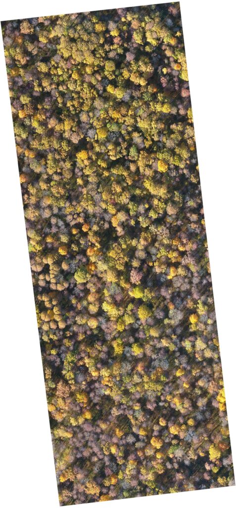
Figure 2. Orthophotomap of the permanent sample plot in the “Kaluzhskie Zaseki” State Nature Reserve (based on aerial survey materials dated 10.10.2021; quadrocopter DJI Phantom 4 Advanced, flight altitude is 117 m)
At the permanent sample plot in the “Kaluzhskie Zaseki” State Nature Reserve the following field surveys of the tree layer were conducted:
- Multiseasonal aerial survey of tree stands using DJI Phantom 4 and DJI Phantom 4 Pro quadcopters) in order to create orthophotomaps of the permanent sample plot.
- Mapping of tree stands by triangulation method based on measuring distances between focal trees (taking into account their trunk radius) and reference points with known coordinates using a laser rangefinder.
Studies of the grass-shrub layer included sampling of dominant grass-shrub species to obtain data on carbon and nitrogen content in different organs of vegetative plants and in plant litter.
Soil cover studies included the study of spatial distribution of organic matter characteristics (Corg, Ntotal, C:N) of forest litter and upper organomineral horizon of soils depending on the location of trees of different species, crown density and dominant species of ground cover.
Main results of field studies
Study of spatial and species structure features of tree layer in multispecies stands
The purpose of field studies of the spatial structure, species-specific growth parameters and dynamics of the tree layer was to obtain data necessary to modify the sub-model of initial tree placement, the sub-model of competition for photosynthetically active radiation (PAR) and the sub-model of tree biomass production and its distribution among organs, taking into account possible crown asymmetry. The main focus of our studies is on analyzing the relationships between spatial and demographic aspects of tree stand dynamics. This is due to the tree placement and size characteristics which are the result of current demographic changes in the plant community and past ecological processes, and competition between trees of different ontogenetic states and size classes is asymmetric.
The data on the location (coordinates) of trunk bases and crown projection centroids of the upper layer trees obtained during field studies on a permanent sample plot in the Prioksko-Terrasny Reserve were used to analyze the nature of their spatial distribution (Shanin et al., 2018), similar to the methodology used in earlier studies (Shanin et al., 2016). The spatial distribution of trunk bases was estimated to be consistent with the random placement model, but the value of the agreement measure with the null hypothesis of random placement (p=0.058) was close to the critical value of 0.05, suggesting that real tree placement has spatial characteristics that deviate from those for completely random, which may suggest some evidence of uniformity. Additional graphical analysis of the L‑function showed for the studied stand a low occurrence of tree pairs with distances between the bases of their trunks of 4–6 meters, which is atypical for random placement. Analysis of the spatial distribution of centroids (geometric centers) of crown projections showed that their location, on the contrary, differed significantly from random towards more regular (p=0.032). Deviation from random placement was associated with a small contribution to the total distribution of short distance pairs (1.5–2.5 m). The regularity of the location of crown projection centroids in space at random location of trunk bases shown for the studied stand, which was also noted in other studies (Sekretenko, 2001; Schröter et al., 2012), reflects the mechanism of tree adaptation to competition from neighbors, which is manifested in asymmetric horizontal growth of crowns in different directions. In trees with different growth strategies, the value of asymmetry manifests itself differently. It is higher in reactive and tolerant species and lower in competitive species, which implies the need for appropriate species-specific parameterization in the model. It should be noted that due to this adaptation mechanism, multispecies stands are able to maintain a high level of phytomass production, maximizing the use of available resources.
Measurements of tree crown projection areas made during field studies showed their expansion towards open areas (Fig. 3), which are formed by “gaps” in the forest canopy as a result of fallen trees of the upper layer. This and the fact that spatial heterogeneity of ecological conditions under the forest canopy is associated with the formation of windthrow gaps (Eastern European forests …, 2004; Bobrovsky, 2010), determined our attention to the problem of studying the spatial features of location and estimation of the area of windthrow gaps in uneven-aged stands of complex species composition.
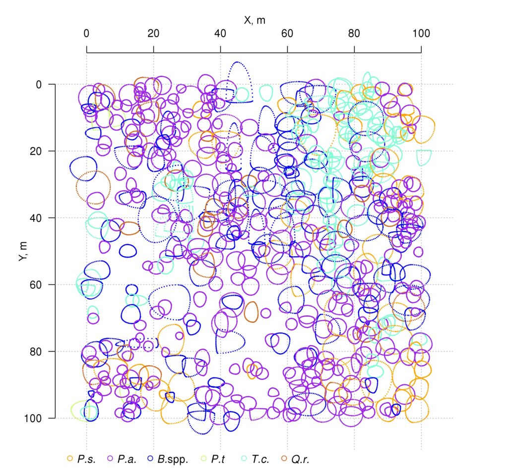
Figure 3. Plan-scheme of tree crown projections at the permanent sample plot of the Prioksko-Terrasny Reserve. The following species are shown in color: P.s. — Pinus sylvestris, P.a. — Picea abies, B.spp. — Betula spp., P.t. — Populus tremula, T.c. — Tilia cordata, Q.r. — Quercus robur
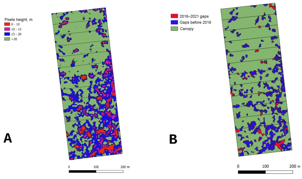
Based on the results of aerial photography of a permanent sample plot in the “Kaluzhskie Zaseki” Nature Reserve, the distribution of forest canopy surface heights was analyzed. This made it possible to identify, determine the size and estimate the proportion of windthrow gaps of different ages in the tree canopy (Fig. 4).
Field studies at the permanent sample plot in the “Kaluzhskie Zaseki” Nature Reserve also included re-census, which provided data on the dynamics of the main characteristics of the stand over a 30‑year period (from 1988 to 2018). The results of comparative analysis showed a marked increase in the average diameter of trees of light-demanding species (Quercus robur, Fraxinus excelsior, Populus tremula and Betula spp.). In shade-tolerant species (Ulmus glabra, Tilia cordata, Acer platanoides), the average diameter increased insignificantly or even decreased over the same period of time, but the total number of trees of these species increased, indicating their successful regeneration under the canopy in conditions of relatively limited PAR resources. The findings are important for analyzing and interpreting the results of simulation evaluations, as well as validating the model system at a qualitative level.
Study of different tree species surface litter spatial distribution
Peculiarities of distribution of needle/leaf and other fractions of litter in the space of forest biogeocenosis are an important factor in the formation of heterogeneity (patchiness) of soil conditions (Orlova et al., 2011). To parameterize the function used in the developed model system to describe the spatial distribution of needle/leaf litter of the tree layer, 12 sets of litter traps with a collection area of 0.25 m2 (0.5 × 0.5 m) under trees of Pinus sylvestris, Picea abies, Betula spp., Quercus robur, Tilia cordata, Acer platanoides species (2 series for each species) were installed at the key plot in the Prioksko-Terrasny Reserve. To install litter traps, trees were selected where the distance from the nearest tree of the same species was at least 100% of the height of the tallest of the trees (either the focal tree or the tallest of the neighboring trees of the same species). Each set of 5 litter catchers was placed along a transect directed away from the focal tree at distances corresponding to 0.050, 0.125, 0.250, 0.500, and 1.000 focal tree heights. The location of all trees with crown projections overlapping the transect was recorded. The litter was sampled once a month. Focal tree litter was sorted into the following fractions: foliage or needles; branches and bark; other (seeds, cones, bud scales, etc.). Tree litter from other species was not separated into fractions. Analysis of the obtained data on the spatial distribution of needle/leaf litter (Fig. 5) showed that the bulk of the litter reaching the soil surface accumulates at a distance of up to 0.125–0.250 of the height of the corresponding tree. The nature of its distribution is determined by the properties of leaves and needles of trees of different species, primarily their specific mass. Among the species studied, the greatest relative range of dispersal is characteristic of Betula spp. and the least is characteristic of Picea abies. No pronounced regularities were found in the distribution of other fractions of the litter.
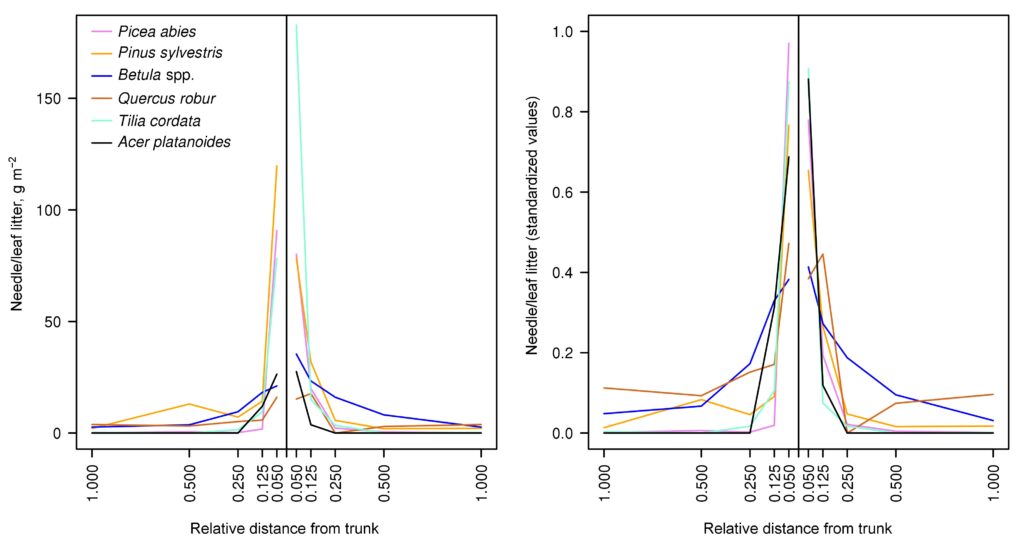
Figure 5. Spatial distribution of needle/leaf litter of trees of different species: left — absolute units; right — values standardized with respect to the total amount of litter for the entire transect
Studies of undergrowth dynamics and regeneration of tree species
Demographic study of undergrowth (trees with trunk diameter less than 6 cm) was carried out in the Prioksko-Terrasny Reserve on 5 survey plots 20 × 20 m in size, laid out within the permanent sample plot. Quantitative data were obtained showing the predominance of late successional species of Tilia cordata, Quercus robur, Picea abies and the presence of Acer platanoides in small quantities. Early successional species Pinus sylvestris and Betula spp. were represented only by juvenile and immature individuals, while Populus tremula juveniles were not detected, despite the presence of generative trees of this species in the upper layer of the stand. The results obtained for the permanent sample plot of the Prioksko-Terrasny Reserve reflect the peculiarities of the stage of successional development of forest stands characteristic of the coniferous-broadleaved forest subzone (after fellings or severe fires), when early-successional species are replaced by late-successional ones (Successional Processes …, 1999). Analysis of contingency tables (Vergarechea et al., 2019) showed that undergrowth of Tilia cordata was underrepresented in plots dominated by Betula spp. in the stand and Calamagrostis arundinacea and Pteridium aquilinum in the ground cover. For Picea abies and Quercus robur, on the contrary, such conditions are favorable. At the same time, undergrowth of Picea abies and Quercus robur is poorly represented in areas dominated by Pinus sylvestris in the canopy and Convallaria majalis in the ground layer, while such conditions are favorable for the development of Tilia cordata undergrowth. In areas dominated by Betula spp. in the canopy and Vaccinium myrtillus L. in the living ground cover, Quercus robur undergrowth is poorly represented.
Study of growing conditions, species, spatial structure and dynamics of the forest communities’ grass-shrub layer
The aim of the study was to obtain experimental data necessary to refine the algorithms and parameterization of the living ground cover submodel, which allows modeling the structural and functional organization and population dynamics of ground cover plants, as well as their contribution to the biogenic cycling of elements in forest ecosystems. The main part of studies of this thematic block was carried out on the territory of Prioksko-Terrasny Reserve and in its surroundings; the objects of study were dominant species of the grass-shrub layer of coniferous-broad-leaved and broad-leaved forests.
Determination of species tolerance ranges to light and soil moisture factors
The objects of research are Aegopodium podagraria, Calamagrostis arundinacea, Carex pilosa L., Convallaria majalis, Oxalis acetosella L., Pteridium aquilinum, Vaccinium myrtillus, Vaccinium vitis–idaea L. To evaluate the ranges of plant tolerance to light (Table 1), temporary sample plots were laid out for the cenopopulation of each species under extreme light conditions. The transmittance of solar radiation through the forest canopy (Global Light Index, GLI) was determined at the level of photosynthetic plant organs. Circular hemispherical photographs were taken at the zenith using a Canon EOS 600D camera with a Sigma AF 4.5/2.8 EX DC HSM Fisheye lens with a 180 degree angle of view. The top of the frame was oriented to true north, taking into account magnetic declination.
To determine the ranges of plant tolerance to soil moisture (Table 1), temporary sample plots were laid out for the cenopopulation of each species under extreme moisture conditions. Moisture measurements were taken multiple times under different weather conditions. Soil moisture data were obtained using an MG‑44 soil moisture meter with a 4‑electrode sensor (at least 15 measurements for each temporary sample plot at each measurement period).
Table 1. Ranges of tolerance of grass-shrub plant species to light and soil moisture factors
| Species | Litter moisture tolerance range (vol. %) | Light tolerance range (GLI, %) |
| Aegopodium podagraria | 5.2–25.3 | 0.3–10.3 |
| Calamagrostis arundinacea | 1.5–29.3 | 1.1–22.4 |
| Carex pilosa | 7.4–26.9 | 0.4–28.6 |
| Convallaria majalis | 5.3–33.7 | 0.9–24.0 |
| Oxalis acetosella | 7.2–29.9 | 0.3–8.6 |
| Pteridium aquilinum | 3.2–24.8 | 2.1–30.9 |
| Vaccinium myrtillus | 5.7–61.1 | 0.4–27.5 |
| Vaccinium vitis–idaea | 4.9–46.8 | 0.4–31.9 |
Determining the effect of conditions patchiness created by trunks and crowns of different species trees on soil moisture and illumination at the level of grass-shrub layer.
For cenopopulations of Calamagrostis arundinacea, Convallaria majalis, Pteridium aquilinum, Vaccinium myrtillus, Vaccinium vitis-idaea, 5 microsites were laid out along transects from the trunk of one tree to the trunk of the neighboring tree (2 in the clumping part, 2 under tree crowns and 1 in the inter-crown space). Soil moisture measurements and estimates of solar radiation transmittance through the forest canopy were made at each of the microsites (Fig. 6). At the same microsites, samples of forest litter and upper root-inhabitable layer of soil were taken to determine their nitrogen and carbon content.
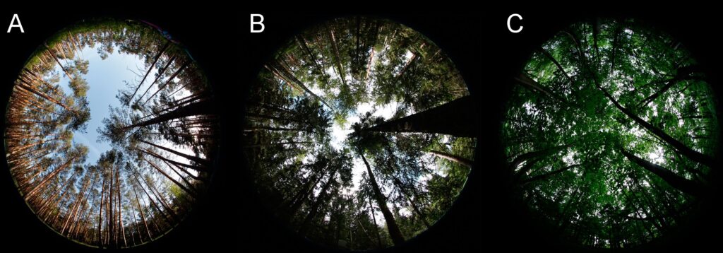
Figure 6. Images of light transmission by crowns of different densities (A — sparse, B — medium density, C — dense)
Determination of photosynthesis intensity dependence on soil moisture under controlled experiment
The studies were conducted on a 1 × 1 m temporary sample plot where Pteridium aquilinum, Calamagrostis arundinacea, and Convallaria majalis grew together. One week before the experiment, WatchDog moisture loggers with two WaterScout SM‑300 moisture sensors (1 in the forest floor and 1 in the mineral horizon at a depth of 5 cm from the lower boundary of the floor) were installed in the trial area. Additionally, temperature sensors were installed (on the soil surface, in the forest floor and in the mineral soil at depths of 10 and 20 cm). On August 12, 2019, between 10 am and 11:30 am, 212 liters of water were applied to the sample plot, which approximately corresponded to the precipitation rate for 3 summer months for the area. To prevent additional wetting of the sample plot during the experiment, the site was covered with an awning fixed at a height of 1.5 m. Three leaves (i.e., 9 measurement points) were selected on plants of each species, and photosynthetic intensity measurements were taken at each of the 9 points in turn over the course of a day (from 11:30 am on August 12, 2019 to 11:30 am on August 13, 2019) with no breaks between measurements (repeated at the end of the measurement cycle). Photosynthesis rates were determined with a PAR‑FluorPen FP 110D fluorimeter. The readings of soil moisture sensors were recorded automatically at 15 min intervals, temperature sensors were recorded manually at 1 h intervals. In parallel, air temperature and humidity were recorded every hour using an aspiration psychrometer. After the daily cycle of measurements, single measurements at 9 points were repeated every 3 days until the end of the growing season using a similar methodology.
In addition, the parameters of photosynthesis intensity of dominant species response function of the grass-shrub layer to changes in air temperature and moisture of forest floor and root-inhabitable layer of soils were determined at several sample plots (Fig. 7). Photosynthetic rates were determined on sample plots during the 2018–2021 growing seasons under different soil temperature and moisture conditions. More than 3,000 measurements have been made. The root layer moisture was determined by a soil moisture meter with preliminary calibration for soils differing in granulometric composition. At each sample plot, one-time measurements were performed in 15‑fold repetition, due to the large variability of this indicator. Temperature was measured over a range of conditions from −2 ºC to +27 ºC (IT‑8 instrument) for air once per survey cycle for each sample plot, for soil it was in a threefold repetition.
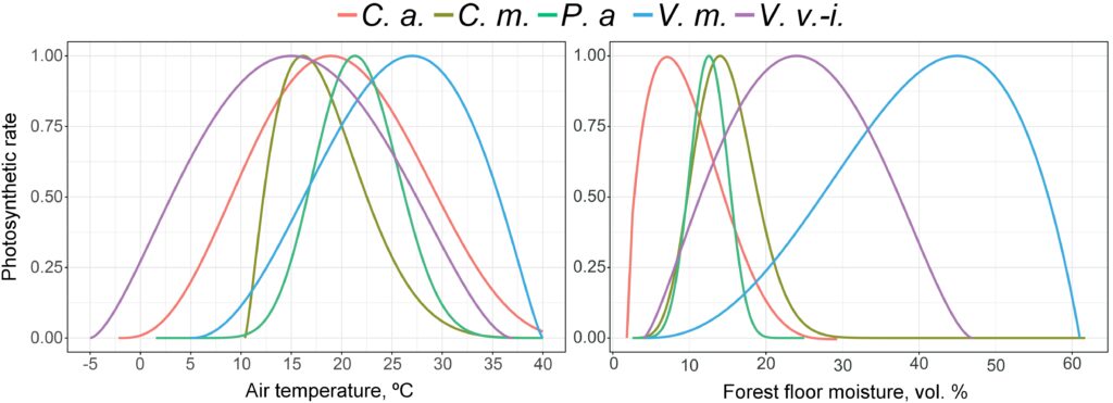
Figure 7. Photosynthesis intensity response functions of dominant species of the grass-shrub layer to changes in air temperature and forest forest floor moisture. C. a. — Calamagrostis arundinacea, C. m. — Convallaria majalis, P. a. — Pteridium aquilinum, V. m. — Vaccinium myrtillus, V. v.-i. — Vaccinium vitis-idaea
Studies on the dynamics of plant growth and development during ontogenesis
The objects of study were Aegopodium podagraria, Calamagrostis arundinacea, Carex pilosa, Convallaria majalis, Oxalis acetosella, Pteridium aquilinum. Sample plots were laid in 2018–2020 in areas dominated by these species. Mapping of Calamagrostis arundinacea plants (54 p plants), partial shrubs of Carex pilosa (20 plants) and underground shoots of long-rooted plants Aegopodium podagraria (10 plants), Convallaria majalis (15 plants), Oxalis acetosella (15 plants), Pteridium aquilinum (20 plants) for rhizome growth studies was carried out. Fragments of Oxalis acetosella underground shoots with live leaves were ringed with thin metal wire with orange plastic number tags. The shoots of the other plants were spotted with blue plastic tags stuck next to the shoot in the ground. Twice, in spring and fall, the length of internodes on the shoot, the number of buds and leaves, the length of leaf petiole for each leaf, and the size of horizontal projection of the surface of each leaf plate on the ground surface in two perpendicular directions were measured in the studied plants. For Oxalis acetosella, the number of flower-bearing buds per shoot was additionally noted. The shoots were recorded. Since Carex pilosa leaves remain viable in winter, a special method was developed to determine the timing of their die-off. Squares with a side of 30 cm were cut from the covering material, which corresponds to the size of the above-ground part of Carex pilosa partial shrubs. Holes with a diameter of 10 cm were made in the center of the squares. The resulting “apron” was put on a partial shrubs and secured to the ground on four sides with blue plastic number tags. At each observation period, the number of vegetative and generative shoots, the number of living leaves, and the number of dead leaves were counted for each partial shrub. The whole length and the living part of the leaf were measured for living leaves. Number of generative shoots was counted. Additionally, fragments of all plants excavated for calculating organ rank distributions were measured and recorded.
Determination of plant organs allometric relations
Plants of Aegopodium podagraria, Calamagrostis arundinacea, Carex pilosa, Convallaria majalis, Oxalis acetosella, and Pteridium aquilinum were selected for calculation of allometric ratios. Calamagrostis arundinace specimens (20 specimens) were sampled whole. For Aegopodium podagraria, Carex pilosa, Convallaria majalis, and Oxalis acetosella, plant fragments were sampled on 0.25 m2 microsites (12–25 microsites for each species). For Pteridium aquilinum, 24 plant fragments were excavated from an area of 0.5 × 1.5 m, as well as the whole plant from an area of 0.5 × 8.0 m (Fig. 8). The root systems of all plants were dug out of the soil as gently as possible, after which the roots were washed in running water. In the laboratory, all plant fragments were measured and recorded and then divided into organs, which were weighed after being dried to a completely dry state.
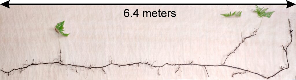
Figure 8. Determination of Pteridium aquilinum rhizome size
Determination of nitrogen content in plant organs and root-inhabitable soil horizons
Along with the determination of allometric ratios, carbon and nitrogen contents were determined in phytomass samples of different plant organs (by high-temperature combustion of samples in a CHN-analyzer). At the same time with plants, samples of forest floor and mineral soil layer corresponding to the species under study were taken at their growing sites, in which carbon and nitrogen content was also determined.
Studies on spatial heterogeneity of soil conditions under the forest canopy
Monitoring of temperature and moisture of forest floor and upper mineral soil horizons, and precipitation as indicators of microclimatic conditions under the forest canopy
Year-round temperature (T) measurement of forest floor and upper mineral soil horizons was carried out starting from November 11, 2016, using two-channel temperature recorders EClerk-USB-2Pt-Kl (“Relsib” production, measurement range is −50… +200 °C, accuracy is ±0.5 °C). Temperature was recorded at intervals of once per hour by sensors located at the boundary of forest floor and soil organomineral horizon and in the soil at a depth of 10 cm. In order to evaluate the influence of crowns of different tree species on soil surface shading, the recorders were installed in series for the following pairs of trees: “Picea abies — Pinus sylvestris“, “Pinus sylvestris — Pinus sylvestris“, “Picea abies — Picea abies“, “Pinus sylvestris — Betula spp. ” and “Betula spp. — Picea abies“. The recorders were with 5 sensors in each series (2 near the trunk bases, 2 under crowns, 1 in the inter-crown space). Moisture was measured on three of the five series. They were “Picea abies — Pinus sylvestris“, “Pinus sylvestris — Betula spp. ” and “Betula spp. — Picea abies“; precipitation was measured on them during the warm season. Registration of precipitation and soil moisture, started on August 28, 2018, was carried out by automatic loggers WatchDog 1400 with Watchdog Tipping Bucket Rain Gauge and WaterScout SM 100 soil moisture sensors (Spectrum Technologies Inc., USA). Moisture sensors were installed in the forest floor and soil horizons at depths of 5 and 15 cm from the lower boundary of the floor. When analyzing the results of hydrothermal parameters measurements, the central point of each series (in the inter-crown space) was taken as the base point, and the difference of parameters with the base point was calculated for the other four points. The results of analyzing data on temperature (T) distribution at the boundary between the forest floor and the organomineral horizon showed no noticeable deviations of T under crowns and near the trunk base from T in the inter-crown space. For soil T at a depth of 10 cm during the warm period of the year, a relative decrease was observed under Picea abies compared to the inter-crown space. In addition, forest floor moisture under Picea abies crowns was on average lower and under Pinus sylvestris crowns higher than in areas between crowns (Fig. 9). These patterns were absent in the mineral soil at depths of 5 and 15 cm. Data from monitoring of soil hydrothermal conditions confirm the importance of taking into account in the sub-model of soil organic matter dynamics of the tree location of different species with correction factors of species-specific decomposition of litter dependence on forest floor moisture.
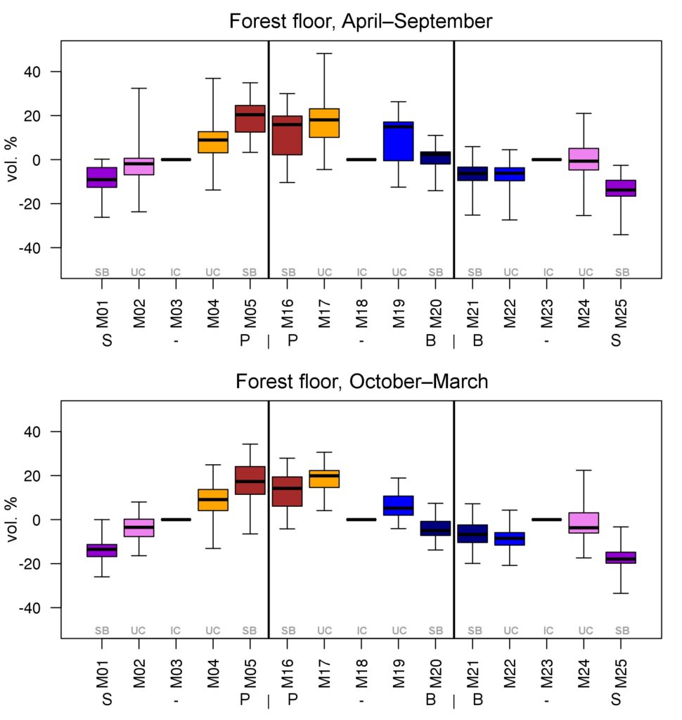
Figure 9. Variation of forest floor moisture content deviations under trees (“SB” — at the trunk base, “UC” — under the crown) from inter-crown areas (“IC”) in warm and cold periods of the year. S — Picea abies, P — Pinus sylvestris, B — Betula spp. Median (thick horizontal line), 1st and 3rd quartiles (“boxes”) and range (“whiskers”) are shown
Analysis of organic matter characteristics spatial heterogeneity (Corg and Ntotal) in soils depending on the species structure of tree layer and ground cover
Soil surveys were conducted according to a unified methodology in August 2018 at key sites in the “Kaluzhskie Zaseki” Nature Reserve and Prioksko-Terrasny Nature Reserve. In order to account for the influence of dominant tree species and ground cover on soil organic matter distribution, forest floor (O) and humus (AY) horizons were sampled along transects between two neighboring trees in a series of 5 points (similar to monitoring of hydrothermal conditions and geobotanical surveys). On a permanent sample plot in the “Kaluzhskie Zaseki” Nature Reserve, 10 transects for pairs of trees were laid out taking into account the multispecies composition of the forest stand. They were “Tilia cordata — Quercus robur“, “Tilia cordata — Betula spp. “, “Tilia cordata — Populus tremula“, “Tilia cordata — Acer platanoides“, “Quercus robur — Acer platanoides“, “Quercus robur — Populus tremula“, “Quercus robur — Fraxinus excelsior“, “Fraxinus excelsior — Acer platanoides“, “Fraxinus excelsior — Betula spp. “, “Ulmus glabra — Ulmus glabra“. At a permanent sample plot in the Prioksko-Terrasny Nature Reserve 7 following transects were selected with different combinations of pairs of predominant tree species of the upper layer: Pinus sylvestris, Picea abies and Betula spp. The thickness of forest floor (cm) was recorded during sampling at a permanent sample plot in the Prioksko-Terrasny Nature Reserve. At the permanent sample plot in the “Kaluzhskie Zaseki” Nature Reserve, the thickness of forest floor at the time of sampling at all points did not exceed 1 cm. The results of the research have been partially published by Priputina et al. (2020).
Soil cover in the mixed coniferous-broadleaved forest community (permanent sample plot in the Prioksko-Terrasny Nature Reserve) shows an increase in forest floor thickness from inter-crown to undercrown spaces and trunk bases, reflecting the intensity of needle/leaf litter input, as confirmed by litter traps’ data. The Corg and Ntotal contents in the O horizon ranged from 17.6–44.9 and 0.84–1.79%, while in the AY horizon they ranged from 0.71–8.5 (Corg) and 0.035–0.33% (Ntotal). The higher variation of indicators was characteristic of the AY horizon, including the relationship between the Ntotal content in soil and the nitrogen status of dominant species of the grass-shrub layer in samples from inter-crown spaces. In the soil of a polydominant stand of broadleaved forest (permanent sample plot in the “Kaluzhskie Zaseki” Nature Reserve), the Corg content in the O horizon averaged 25–30%; elevated values of Corg (40–45%) were under crowns of Betula spp. and Ulmus glabra, and minimum values were under crowns of Tilia cordata (20%). In addition, increased variability in Corg values was shown for the O horizon of the inter-crown sections. In the AY horizon, the Corg content was 1.3–3.5%. For Quercus robur, Tilia cordata and Fraxinus excelsior, the values of Corg content in the humus horizon under crowns were lower than in trunk areas, while for other tree species this pattern was not observed. The Ntotal content in the O horizon averaged 1.0–1.5%, and in the AY horizon it was 0.15–0.20%. The variation of Ntotal content in permanent sample plot in the “Kaluzhskie Zaseki” Nature Reserve soil was markedly lower than that of Prioksko-Terrasny Nature Reserve. The relationships of Corg and Ntotal content in soils with the character of vegetation cover of tree and grass-shrub layers revealed in the course of soil studies reflect the peculiarities of spatial localization and qualitative characteristics of surface and in-soil litter and conditions of its transformation under the influence of hydrothermal conditions formed under the forest canopy (Dhiedt et al., 2022).
BRIEF DESCRIPTION OF THE MODEL SYSTEM
The EFIMOD3 model system is implemented in the statistical programming language R v. 4.1.3 (R Core Team, 2014) and includes the following basic blocks (submodels): initial microrelief; initial tree placement; competition for photosynthetically active radiation (PAR) and soil nitrogen in plant-available forms; tree biomass production and its distribution among organs; spatial distribution of surface and in-soil plant litter; soil organic matter dynamics; hydrothermal conditions in soil; and grass-shrub layer dynamics.
The model system operates with an annual time step (the internal interval of individual submodels or individual procedures may be more detailed such as monthly, daily, or hourly; here we refer to the discreteness in time with which the state output variables are calculated) on a square simulation plot divided into square cells (hereinafter also referred to as “simulation grid” or “simulated site”). The maximum size of the simulation grid is 100 × 100 m (1 ha); the cell size can be arbitrary and was assumed to be 0.5 × 0.5 m in most subsequent simulations with the model system. To avoid edge effects, a torus-closure technique is used, which assumes that cells at the edge of the simulated site that have no neighbors on one or two sides use cells on the opposite edge as neighbors (Haefner et al., 1991). General scheme of the model system is presented in Fig. 10. A brief description of the submodel algorithms is given below; more detailed descriptions of the algorithms, as well as descriptions of the procedures for parameterization, validation, and sensitivity analysis of submodels, are given in the publications cited below. The list of model system parameters is given in Tables 2–5.
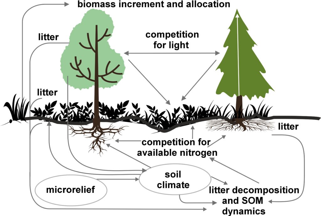
Figure 10. General scheme of the model system
Table 2. Species-specific parameters of competition for soil mineral nitrogen submodel (reproduced from (Shanin et al., 2015a), as amended)
| Ps | Pa | Ls | As | Bp | Pt | Qr | Tc | Fs | Ap | Ug | Fe | |
| aavg | 13.30 | 9.01 | 9.04 | 13.42 | 15.57 | 14.72 | 8.31 | 9.86 | 9.64 | 8.42 | 10.75 | 12.21 |
| bavg | 4.50 | 4.51 | 4.69 | 4.37 | 8.01 | 6.22 | 18.74 | 12.44 | 19.42 | 5.67 | 6.04 | 5.02 |
| cavg | 0.060 | 0.160 | 0.155 | 0.072 | 0.095 | 0.110 | 0.141 | 0.088 | 0.078 | 0.091 | 0.064 | 0.102 |
| amax | 14.84 | 11.99 | 12.02 | 15.50 | 22.11 | 18.05 | 10.24 | 12.71 | 10.98 | 10.26 | 13.24 | 14.02 |
| bmax | 2.77 | 3.13 | 3.22 | 2.84 | 6.64 | 5.22 | 9.76 | 7.78 | 12.62 | 3.54 | 3.62 | 3.78 |
| cmax | 0.068 | 0.190 | 0.186 | 0.081 | 0.110 | 0.140 | 0.153 | 0.094 | 0.080 | 0.092 | 0.068 | 0.112 |
| FRff | 0.033 | 0.050 | 0.039 | 0.048 | 0.029 | 0.031 | 0.034 | 0.032 | 0.027 | 0.034 | 0.048 | 0.026 |
| SRff | 0.036 | 0.053 | 0.041 | 0.051 | 0.031 | 0.029 | 0.036 | 0.034 | 0.028 | 0.035 | 0.050 | 0.030 |
| mstrat | 0.8 | 1.4 | 1.1 | 1.1 | 1.2 | 1.2 | 0.9 | 1.0 | 1.2 | 1.0 | 1.0 | 0.9 |
| aur | 0.226 | 0.108 | 0.215 | 0.122 | 0.138 | 0.119 | 0.101 | 0.097 | 0.112 | 0.161 | 0.115 | 0.140 |
| bur | 0.023 | 0.022 | 0.024 | 0.022 | 0.021 | 0.021 | 0.020 | 0.020 | 0.020 | 0.020 | 0.020 | 0.021 |
Note: Ps — Pinus sylvestris, Pa — Picea abies, Ls — Larix sibirica, As — Abies sibirica, Bp — Betula pendula Roth / Betula pubescens Ehrh., Pt — Populus tremula, Qr — Quercus robur, Tc — Tilia cordata, Fs — Fagus sylvatica, Ap — Acer platanoides, Ug — Ulmus glabra, Fe — Fraxinus excelsior. aavg, bavg, cavg — parameters of the equation describing the average range of horizontal root spread as a function of tree size; amax, bmax, cmax — similarly for the maximum range of horizontal spreading of roots (Laitakari, 1927, 1934; Bobkova, 1972; Verkholantseva, Bobkova, 1972; Lashchinsky, 1981; Diagnoses and keys …, 1989; Kajimoto et al., 1999; Kalliokoski et al., 2008, 2010a, 2010b; Terekhov, Usoltsev, 2010; Kalliokoski, 2011); FRff — parameter describing the dependence of the fraction of fine roots in the forest floor on its thickness; SRff — similarly for skeletal roots (Kalela, 1949, 1954; Bobkova, 1972; Verkholantseva, Bobkova, 1972; Baneva, 1980; Lozinov, 1980; Laschinsky, 1981; Abrazhko, 1982; Majdi, Persson, 1993; Persson et al., 1995; Braun, Flückiger, 1998; Thomas, Hartmann, 1998; Rust, Savill, 2000; Rothe, Binkley, 2001; Schmid, 2002; Veselkin, 2002; Puhe, 2003; Brandtberg et al., 2004; Leuschner et al., 2004; Oostra et al., 2006; Püttsepp et al., 2006; Withington et al., 2006; Helmisaari et al., 2007, 2009; Ostonen et al., 2007; Tanskanen, Ilvesniemi, 2007; Tatarinov et al., 2008; Dauer et al., 2009; Meinen et al., 2009; Yuan, Chen, 2010; Giniyatullin, Kulagin, 2012; Peichl et al., 2012; Usoltsev, 2013a; Brunner et al., 2013; Chenlemuge et al., 2013; Hansson et al., 2013; Urban et al., 2015; Grygoruk, 2016; Jagodzinski et al., 2016; Takenaka et al., 2016; Tardío et al., 2016; Mauer et al., 2017; Meier et al., 2018; Zhang et al., 2019; Wambsganss et al., 2021); mstrat — a multiplier describing the change in vertical distribution of root biomass in the presence of trees of other species (with values less than 1 the root system becomes deeper, with values greater than 1 it becomes more surfaced) (Büttner, Leuschner, 1994; Schmid, 2002; Schmid, Kazda, 2002; Bolte, Villanueva, 2006; Kelty, 2006; Kalliokoski et al., 2010a, 2010b; Richards et al., 2010; Brassard et al., 2011; Shanin et al., 2015b; Goisser et al., 2016; Jaloviar et al., 2018; Aldea et al., 2021); aur — specific nitrogen consumption by roots of annual trees, gram of nitrogen per kg of fine root biomass per day; bur — parameter describing the decrease in specific nitrogen consumption with tree age (Gessler et al., 1998; Lebedev, Lebedev, 2011, 2012; Lebedev, 2012a, 2012b, 2013; Guerrero‑Ramírez et al., 2021).
Table 3. Species-specific parameters of competition for PAR submodel (reproduced from (Shanin et al., 2020), as amended)
| Ps | Pa | Ls | As | Bp | Pt | Qr | Tc | Fs | Ap | Ug | Fe | |
| SHP | EL | CN | CN | CN | SE | SE | CY | SE | SE | EL | SE | EL |
| α | 3.788 | 2.519 | 3.650 | 2.614 | 2.254 | 2.324 | 2.727 | 2.816 | 2.918 | 2.798 | 2.824 | 3.421 |
| ε | 1.283 | 1.448 | 1.262 | 1.422 | 1.386 | 3.392 | 1.656 | 1.700 | 1.316 | 1.702 | 1.714 | 1.186 |
| γ[e−2] | −8.38 | −4.71 | −7.52 | −4.82 | −6.42 | −6.05 | −5.48 | −5.22 | −4.22 | −5.66 | −5.12 | −7.55 |
| μ | 0.724 | 0.926 | 0.712 | 0.888 | 0.682 | 0.715 | 0.694 | 0.702 | 0.816 | 0.688 | 0.710 | 0.615 |
| υCR | 8.882 | 5.757 | 7.955 | 5.402 | 9.147 | 8.412 | 11.178 | 9.120 | 10.912 | 9.064 | 8.842 | 8.764 |
| υCL | 38.167 | 45.420 | 41.714 | 46.166 | 52.571 | 46.271 | 42.718 | 42.172 | 45.212 | 43.224 | 41.716 | 37.162 |
| ηCR[e−2] | −2.04 | −4.82 | −3.02 | −4.22 | −2.54 | −2.61 | −3.04 | −2.71 | −3.12 | −3.14 | −3.22 | −2.81 |
| ηCL[e−2] | −1.37 | −2.43 | −1.64 | −2.49 | −1.42 | −1.55 | −1.49 | −1.88 | −2.52 | −1.96 | −1.78 | −1.32 |
| κCR[e−6] | −4.46 | −1.62 | −3.91 | −1.78 | −4.78 | −4.91 | −3.12 | −2.74 | −1.51 | −2.14 | −1.88 | −4.31 |
| κCL[e−6] | −8.92 | −4.86 | −4.22 | −4.81 | −5.39 | −4.67 | −3.47 | −3.20 | −3.00 | −2.97 | −2.01 | −8.16 |
| σLV | 0.043 | 0.042 | 0.048 | 0.044 | 0.057 | 0.059 | 0.028 | 0.012 | 0.010 | 0.011 | 0.022 | 0.013 |
| σBM | 0.079 | 0.059 | 0.062 | 0.061 | 0.119 | 0.121 | 0.115 | 0.102 | 0.118 | 0.106 | 0.124 | 0.101 |
| τLV | 1.128 | 1.292 | 1.333 | 1.264 | 1.123 | 1.126 | 1.152 | 1.118 | 1.076 | 1.102 | 1.074 | 1.326 |
| τBM | 1.020 | 1.168 | 1.200 | 1.151 | 0.949 | 0.948 | 0.996 | 0.993 | 0.949 | 0.979 | 0.954 | 1.122 |
| ψLV | −3.430 | −2.622 | −2.545 | −2.658 | −3.146 | −3.127 | −3.312 | −3.527 | −3.992 | −3.674 | −3.872 | −2.818 |
| ψBM | −3.596 | −2.589 | −2.428 | −2.602 | −3.907 | −3.878 | −3.622 | −3.722 | −4.061 | −3.840 | −3.912 | −3.022 |
| ωLV | 4.987 | 3.962 | 4.116 | 3.848 | 3.979 | 4.003 | 4.565 | 4.128 | 4.446 | 4.220 | 4.450 | 4.792 |
| ωBM | 3.667 | 2.765 | 2.664 | 2.641 | 3.659 | 3.626 | 4.372 | 4.110 | 4.199 | 4.192 | 4.217 | 4.442 |
| SLV | 8.8 | 5.4 | 4.9 | 9.5 | 18.7 | 17.0 | 17.5 | 22.1 | 21.6 | 23.7 | 24.0 | 16.0 |
| Lmin | 0.340 | 0.015 | 0.320 | 0.010 | 0.290 | 0.180 | 0.105 | 0.010 | 0.008 | 0.010 | 0.010 | 0.050 |
Note: Species codes are according to Table 2. SHP — crown shape (EL — vertically asymmetric ellipsoid, SE — semi-ellipsoid, CN — composite cone, CY — cylinder); α, ε, γ, μ — coefficients of the equation to account for the influence of neighboring trees on the focal tree crown size; υ, η, κ — coefficients of the equation for calculating crown sizes (CR — average radius at the widest part, CL — vertical extent) (Pugachevsky, 1992; Tselniker et al., 1999; Widlowski et al., 2003; Rautiainen, Stenberg, 2005; Lintunen, Kaitaniemi, 2010; Thorpe et al., 2010; Seidel et al., 2011; Usoltsev, 2013b, 2016; Kuehne et al., 2013; Lintunen, 2013; Falster et al., 2015; Pretzsch et al., 2015; Shanin et al., 2016, 2018; Dahlhausen et al., 2016; Danilin, Tselitan, 2016; Barbeito et al., 2017; Pretzsch, 2019; Jucker et al., 2022; Shashkov et al., 2022); σ, τ, ψ, ω — coefficients of the equation of leaf biomass distribution (LV) and total biomass of leaves and branches (BM) in the vertical crown profile (Nosova, 1970; Gulbe et al., 1983; Niinemets, 1996; Èermák, 1998; Jarmiško, 1999; Bobkova et al., 2000; Mäkelä, Vanninen, 2001; Tahvanainen, Forss, 2008; Petriţan et al., 2009; Lintunen et al, 2011; Hertel et al., 2012; Šrámek, Čermák, 2012; Usoltsev, 2013a; Gspaltl et al., 2013; Berlin et al., 2015; Montesano et al., 2015; Hagemeier, Leuschner, 2019a, 2019b; Kükenbrink et al., 2021); SLV — specific one-sided leaf surface area, m2 kg−1 (Ross, 1975; Gulbe et al., 1983; Èermák, 1998; Widlowski et al., 2003; Utkin et al., 2008; Collalti et al., 2014; Thomas et al., 2015; Forrester et al., 2017); Lmin — PAR threshold value, as a fraction of PAR above the canopy (Evstigneev, 2018; Leuschner, Hagemeier, 2020). The marks [e−2] and [e−6] after the parameter names mean that the value given in the table must be multiplied by 10 to the corresponding negative degree to obtain the actual value of the parameter.
Table 4. Species-specific parameters of the biomass production submodel (reproduced from (Shanin et al., 2019), as amended)
| Ps | Pa | Ls | As | Bp | Pt | Qr | Tc | Fs | Ap | Ug | Fe | |
| T0 | 1 | −3 | −5 | −1 | 2 | 5 | 5 | 5 | 3 | 5 | 5 | 5 |
| T1 | 23 | 17 | 24 | 20 | 18 | 20 | 23 | 25 | 22 | 27 | 25 | 25 |
| T2 | 28 | 27 | 29 | 28 | 30 | 32 | 33 | 35 | 34 | 35 | 34 | 33 |
| D0 | 0.82 | 0.50 | 0.56 | 0.52 | 0.63 | 0.71 | 0.55 | 0.59 | 0.64 | 0.53 | 0.48 | 0.72 |
| D1 | 2.20 | 1.36 | 1.62 | 1.41 | 1.72 | 1.88 | 1.44 | 1.62 | 1.75 | 1.12 | 1.22 | 1.86 |
| ψmin | −3.34 | −0.68 | −1.75 | −1.14 | −1.55 | −1.62 | −1.47 | −1.56 | −1.93 | −1.38 | −1.43 | −2.37 |
| CST | 0.474 | 0.504 | 0.467 | 0.497 | 0.494 | 0.496 | 0.484 | 0.472 | 0.469 | 0.471 | 0.465 | 0.463 |
| CBR | 0.498 | 0.522 | 0.477 | 0.519 | 0.501 | 0.518 | 0.491 | 0.475 | 0.464 | 0.477 | 0.471 | 0.460 |
| CLV | 0.507 | 0.532 | 0.474 | 0.535 | 0.512 | 0.528 | 0.504 | 0.474 | 0.462 | 0.458 | 0.467 | 0.466 |
| CSR | 0.461 | 0.486 | 0.471 | 0.506 | 0.502 | 0.499 | 0.486 | 0.501 | 0.454 | 0.438 | 0.445 | 0.435 |
| CFR | 0.504 | 0.527 | 0.476 | 0.522 | 0.508 | 0.522 | 0.502 | 0.506 | 0.484 | 0.492 | 0.499 | 0.484 |
| NST | 1.4 | 1.6 | 1.7 | 2.2 | 2.1 | 2.7 | 3.1 | 2.8 | 2.4 | 2.7 | 2.8 | 2.8 |
| NBR | 3.2 | 4.2 | 3.8 | 5.4 | 6.4 | 6.3 | 6.9 | 7.2 | 6.2 | 5.6 | 7.2 | 6.8 |
| NLV | 11.9 | 14.1 | 13.3 | 16.4 | 23.7 | 23.9 | 24.8 | 28.9 | 20.3 | 19.6 | 28.1 | 23.6 |
| NSR | 2.2 | 3.8 | 2.9 | 3.9 | 6.0 | 5.4 | 5.7 | 6.7 | 5.2 | 5.6 | 7.1 | 6.5 |
| NFR | 3.7 | 5.7 | 5.1 | 6.8 | 7.5 | 8.0 | 8.7 | 7.9 | 7.5 | 7.8 | 9.6 | 9.1 |
| NLIT | 7.0 | 8.6 | 8.1 | 9.8 | 13.3 | 13.6 | 10.1 | 14.9 | 8.1 | 7.9 | 11.2 | 13.3 |
| A1 | 0.70 | 0.95 | 0.90 | 0.95 | 0.90 | 0.90 | 0.60 | 0.60 | 0.70 | 0.60 | 0.65 | 0.60 |
| A2 | 3.00 | 4.00 | 3.50 | 4.00 | 4.00 | 4.00 | 2.25 | 2.50 | 3.00 | 2.50 | 3.00 | 3.00 |
| Amax | 500 | 600 | 600 | 400 | 250 | 200 | 1200 | 600 | 600 | 450 | 350 | 400 |
| Hmax | 50 | 52 | 48 | 44 | 36 | 38 | 42 | 40 | 48 | 40 | 40 | 52 |
| EVG | + | + | − | + | − | − | − | − | − | − | − | − |
| Pmax | 7.72 | 4.61 | 3.26 | 2.55 | 9.10 | 13.29 | 20.20 | 21.08 | 14.20 | 4.54 | 22.97 | 15.52 |
| Km | 245.78 | 224.41 | 374.19 | 177.56 | 139.02 | 305.56 | 283.00 | 286.72 | 236.60 | 135.25 | 351.25 | 302.24 |
| Kbb | 3.55 | 4.56 | 4.00 | 4.00 | 9.36 | 13.50 | 3.30 | 6.00 | 12.70 | 13.56 | 6.00 | 6.00 |
| ρST | 470 | 405 | 425 | 350 | 590 | 380 | 620 | 470 | 560 | 590 | 595 | 675 |
| z | 1.36 | 0.93 | 0.27 | 0.90 | 0.95 | 0.47 | 0.68 | 0.71 | 0.72 | 0.25 | 1.27 | 0.72 |
| y | 0.12 | 0.45 | 5.54 | 0.75 | 0.42 | 2.23 | 0.93 | 0.93 | 1.24 | 3.37 | 0.18 | 1.11 |
| crank | 0.65 | 0.62 | 0.80 | 0.64 | 0.77 | 0.70 | 0.68 | 0.64 | 0.74 | 0.65 | 0.68 | 0.73 |
| drank | −0.21 | −0.20 | −0.19 | −0.20 | −0.23 | −0.28 | −0.30 | −0.28 | −0.29 | −0.29 | −0.31 | −0.28 |
| erank | −1.72 | −0.76 | −0.55 | −0.78 | −1.35 | −1.57 | −0.78 | −0.68 | −1.35 | −0.78 | −0.81 | −1.17 |
| frank | −0.16 | −0.24 | −0.32 | −0.25 | −0.27 | −0.19 | −0.32 | −0.36 | −0.32 | −0.32 | −0.34 | −0.28 |
| DLIT | 0.36 | 0.23 | 0.22 | 0.37 | 0.39 | 0.39 | 0.42 | 0.39 | 0.39 | 0.41 | 0.36 | 0.39 |
Note: Species codes are according to Table 2. T0 — minimum temperature for the production process, °C; T1 — temperature corresponding to the saturation point, above which there is no productivity growth, °C; T2 — temperature of the production process suppression beginning, °C (Niinemets et al., 1999; Dreyer et al., 2001; Medlyn et al., 2002; Peng et al., 2002; Mäkelä et al., 2008; Amichev et al., 2010); D0 — VPD value, up to which its increase does not lead to decrease of stomatal conductance, kPa; D1 — VPD value, at which the stomatal conductance is halved, kPa (Appleby, Davies, 1983; Pigott, 1991; Seidl et al., 2005; Celniker et al., 2007; Gebauer, 2010; Packham et al., 2012; Kharuk et al., 2017; Thomas et al., 2018); ψmin —soil moisture threshold value, MPa (Jarvis, 1976; Hinckley et al., 1978; Appleby, Davies, 1983; Ranney et al., 1991; Bréda et al., 1995; Hanson et al., 2001; Lemoine et al., 2001; Lexer, Hönninger, 2001; Wullschleger, Hanson, 2003; Shein, 2005; Seidl et al., 2005; Niinemets, Valladares, 2006; Saxton, Rawls, 2006; Geßler et al., 2007; Dulamsuren et al., 2008; Köcher et al., 2009; Rötzer et al., 2013; Way et al., 2013); CST — carbon content of the trunk, as a fraction of the absolute dry mass; CBR — the same parameter for branches; CLV — the same parameter for foliage/needles; CSR — the same parameter for skeletal roots; CFR — the same parameter for fine roots (Peñuelas, Estiarte, 1996; Niinemets, Kull, 1998; Balboa‑Murias et al., 2006; Iivonen et al., 2006; Sinkkonen, 2008; Hansson et al., 2010; Dymov et al., 2012; Peichl et al., 2012; Uri et al., 2012, 2019; Deineko, Faustova, 2015; Medvedev et al., 2015; Giertych et al., 2015; Steffens et al., 2015; Zadworny et al., 2015; Zhu et al., 2017; Tumenbaeva et al., 2018; Koshurnikova et al., 2018; Betekhtina et al., 2019; Kaplina, Kulakova, 2021); NST — specific nitrogen consumption per trunk mass unit growth, grams of nitrogen per 1 kg of growth; NBR — the same parameter for branches; NLV — the same parameter for foliage/needles; NSR — the same parameter for skeletal roots; NFR — the same parameter for fine roots; NLIT — N content in leaf litter, grams of nitrogen per 1 kg of litter (Remezov et al., 1959; Bocock, 1964; Remezov, Pogrebnyak, 1965; Morozova, 1971, 1991; Novitskaya, 1971; Kazimirov, Morozova, 1973; Molchanov, Polyakova, 1974, 1977; Rusanova, 1975; Smeyan et al., 1977; Khavron’in et al., 1977; Luk’yanets, 1980; Rabotnov, 1980; Vakurov, Polyakova, 1982a, 1982b; Vtorova, 1982; Oskina, 1982; Bobkova, 1987; Karmanova et al., 1987; Stolyarov et al, 1989; Nosova, Kholopova, 1990; Migunova, 1993; Lukina et al., 1994; Bauer et al., 1997; Niinemets, 1998; Trémolières et al., 1999; Sudachkova et al., 2003; Peuke, Rennenberg, 2004; Modeling the dynamics of …, 2007; Nahm et al., 2007; Vesterdal et al., 2008; Dannenmann et al., 2009; Hobbie et al., 2010; Vinokurova, Lobanova, 2011; Reshetnikova, 2011; Dymov et al., 2012; Falster et al., 2015; Matvienko, 2017); A1, A2 — regression coefficients of dependence of biomass production on tree height and age; Amax — theoretical maximum possible (for this species) age, years; Hmax — theoretical maximum possible (for this species) height, m (Prentice, Helmisaari, 1991; Landsberg, Waring, 1997; Lexer, Hönninger, 2001; Usoltsev, 2002; Eastern European Forests …, 2004; Seidl et al., 2005; Bobkova et al., 2007; Shvidenko et al., 2008; Praciak, 2013); EVG — whether the species is evergreen or deciduous; Pmax — maximum photosynthesis intensity in terms of carbon, μmol m−2 s−1; Km — PAR intensity, at which 0.5 of the full photosynthesis intensity is reached, μmol m−2 s−1 (Kull, Koppel, 1987; von der Heide‑Spravka, Watson, 1992; Kloeppel, Abrams, 1995; Luoma, 1997; Kazda et al., 2000; Oleksyn et al., 2000; Aschan et al., 2001; Zagirova, 2001; Medlyn et al., 2002; Le Goff et al., 2004; Dulamsuren et al., 2009; Gardiner et al., 2009; Ďurkovič et al., 2010; Suvorova et al., 2017; Gerling, Tarasov, 2020); Kbb — Ball-Berry coefficient for the calculation of the stomatal conductivity (Miner et al., 2017; Pace et al., 2021); ρST — trunk density (including bark), kg m−3 (Reference book …, 1989; Zhang et al., 1993; Luostarinen, Verkasalo, 2000; Kärki, 2001; Mäkinen et al., 2002; Alberti et al., 2005; Heräjärvi, Junkkonen, 2006; Lal et al., 2007; Gryc et al., 2008; Jyske et al., 2008; Kiaei, Samariha, 2011; Tomczak et al., 2011; Luostarinen, 2012; Skarvelis, Mantanis, 2013; Mederski et al., 2015; De Jaegere et al., 2016; Diaconu et al., 2016; Díaz‑Maroto, Sylvain, 2016; Hamada et al., 2016; Zajączkowska, Kozakiewicz, 2016; Liepiņš et al., 2017; Viherä‑Aarnio, Velling, 2017; Giagli et al., 2018); z, y — empirical coefficients for the conversion of tree trunk size to its biomass (Usoltsev, 2002, 2016; Shvidenko et al., 2008); crank, drank, erank, frank — empirical coefficients for calculating tree mass distribution by organs (Stakanov, 1990; Helmisaari et al., 2002; Falster et al., 2015; Usoltsev, 2016; Komarov et al., 2017b); DLIT — parameter characterizing the range of needle/leaf litter dispersion as a function of tree height.
Table 5. General parameters of the model system (reproduced from (Shanin et al., 2015a; Shanin et al., 2019; Shanin et al., 2020), as amended)
| Parameter | Value |
| dT — delayed reaction time to temperature change, days (Mäkelä et al., 2008) | 6 |
| ψfc — soil water potential at the lowest field water holding capacity, MPa (Hanson et al., 2001; Wullschleger, Hanson, 2003; Shein, 2005; Saxton, Rawls, 2006) | −0.033 |
| C0 — base CO2 concentration, ml m−3) (Friedlingstein et al., 1995; Coops et al., 2005; Seidl et al., 2005; Swenson et al., 2005). | 340 |
| Cb — CO2 concentration at the compensation point, ml m−3 (Friedlingstein et al., 1995; Coops et al., 2005; Seidl et al., 2005; Swenson et al., 2005) | 80 |
| β0 — response factor to CO2 concentration (Friedlingstein et al., 1995; Norby et al., 2005) | 0.6 |
| w — weighting factor of combining environmental factors (Frolov et al., 2020a) | 0.5 |
| CRmax — threshold ratio of the maximum crown projection radius to the mean radius (Shanin et al., 2020) | 1.25 |
| Kred — PAR transmittance coefficient by foliage | 0.5 |
| mfert — modifier of the root systems horizontal spread range for oligo-, meso- and eutrophic habitats (Shanin et al., 2015a) | 1.2; 1.0; 0.8 |
| mmoist — modifier of the root systems horizontal spread range for habitats with low, moderate and excessive moisture content (Shanin et al., 2015a) | 1.3; 1.0; 0.9 |
| pa — parameter of probabilistic self-thinning of stands (Seidl et al., 2012) | 0.02 |
| aNmin[L] — parameter of the function for calculating nitrogen mineralization in subhorizons L of organogenic (forest floor) and pools L of organomineral soil horizons for boreal and temperate climates | −1.41; −1.26 |
| aNmin[F] — parameter of the function of calculation of nitrogen mineralization in sub-horizons F and H of organogenic and pool F of organomineral soil horizons for boreal and temperate climates | −0.97; −0.88 |
| aNmin[H] — parameter of nitrogen mineralization calculation function in pool H of soil organomineral horizon for boreal and temperate climates | −1.37; −1.38 |
| bNmin[L] — parameter of nitrogen mineralization calculation function in subhorizons L of organogenic and pools L of organomineral soil horizons for boreal and temperate climates | −105.02; −104.92 |
| bNmin[F] — parameter of nitrogen mineralization calculation function in sub-horizons F and H of organogenic and pool F of organomineral soil horizons for boreal and temperate climates | −103.24; −103.87 |
| bNmin[H] — parameter of nitrogen mineralization calculation function in pool H of soil organomineral horizon for boreal and temperate climates | −104.43; −104.53 |
The input variables of the model system at the initialization stage are as follows: habitat type in terms of trophicity (oligo-, meso- or eutrophic) and moisture content (dry, moderate (normal), wet); geographic coordinates (in decimal degrees); soil granulometric composition (fraction of silt, clay and sand); initial stand parameters (type of tree spatial arrangement (pseudo-random, clustered, regular planting, etc.), density (trees ha−1), species composition, distribution of trees in height and trunk diameter, microrelief parameters (height amplitude, type of heterogeneities; thickness of all considered soil layers (m); bulk density of all considered soil layers (kg m−3); carbon and nitrogen content in sub-horizons L, F and H of organogenic horizon and pools L, F and H of organomineral horizon (kg m−2); soil acidity, soil drainability (logical value, high/low). Input variables of the model system at a single (daily) step are the following: minimum, average and maximum air temperature (°C); water vapor pressure deficit (kPa); relative air humidity (%); precipitation (mm day−1); atmospheric carbon dioxide concentration (ml m−3); nitrogen compound input with precipitation (in terms of nitrogen, kg m−2 day−1). Simulation of felling (parameters include intensity of felling, order of removal of different tree species during felling, amount of felling remains, etc.) and tree planting (parameters: planting density, trees ha−1, species composition, size and spatial location parameters) at certain modeling steps. Model system also has a number of “technical” parameters (size of simulation grid and unit cell of simulation grid; sampling rate of curves describing crown shapes, etc.), which are not deciphered here.
Initialization of the model system
Microrelief
Since microrelief is the result of interaction of a complex set of processes occurring on different spatial scales and with different characteristic times, the construction of a process-based model (i.e., reproducing the real mechanisms of microrelief formation) seems inexpedient. Instead, the microrelief generation algorithm is based on the principle of generating a set of cells with statistical characteristics of relative height distribution given in the form of external parameters of the submodel. For the cell having the smallest value of absolute height, the value of relative height is taken as 0, and for the other cells the height is calculated relative to it (in meters). The algorithm operation includes the following steps: (1) generation of “historical” heterogeneity (the spatial scale of elements is from meters to tens of meters); (2) generation of microheterogeneities (the spatial scale of elements is comparable to the size of the simulation grid cell); (3) generation of heterogeneities associated with the presence of near-trunk elevations and treefall-soil complexes (“hollow, hillock, log”) (Karpachevsky, 1981); (4) generation of the overall slope.
The first step involves the generation of a Gaussian random field (Hristopulos, 2020) with the number of nodes and heterogeneity amplitude (the difference between the maximum and minimum values of the relative cell heights) given as input parameters. During the second stage, the obtained values of relative heights are modified with uniformly distributed random deviations, the amplitude of which is given by the input parameter of the submodel. The procedure for generating tree-base mounds at this stage of submodel development requires their magnitude to depend only on the diameter of the tree trunk at breast level and is assumed to be 0.5 of the latter. The overall slope in the simulated site is calculated using a general plane equation the parameters depending on the azimuth (in degrees relative to the direction to geographic north) and slope magnitude (in %) given as input parameters.
Stand spatial structure
The structure of the model system assumes that the coordinates of each tree correspond to the coordinates of the center of the cell in which the tree is placed, and there cannot be more than one tree in the same cell. The stand spatial structure submodel allows the realization of several types of initial tree placement on the simulated site.
When uniform pseudorandom placement is implemented, tree coordinates are pseudorandomly selected from the available range. Pseudorandom placement with threshold distance is realized in two variants. In the stand density prioritized variant, in the first step the algorithm places a given number of trees as uniformly as possible, using either a Fibonacci grid (Fomin, 1988) or a square grid with some elements skipped. In the second step, the algorithm randomly shifts each tree relative to its original coordinates within a certain distance given by the shift parameter. This parameter defines the maximum distance (in fractions of one unit) from half of the minimum tree spacing at the original regular spacing. In the minimum distance priority variant, the algorithm iteratively tries to place each new tree in such a way that the distance from it to the nearest neighboring tree is not less than the threshold distance (the so-called “hard-core distance”) specified in the submodel parameters. The cycle stops when a threshold number of unsuccessful attempts to find a location to place a new tree is exceeded (Teichmann et al., 2013). Thus, this algorithm may not be able to realize the stand density given in the initial parameters, but it ensures that the minimum distance between neighboring trees is maintained.
Regular tree placement is designed to simulate the artificial plantings and has two parameters: row spacing width and distance between seedlings in a row. When implementing direct tree placement, these parameters are discretized with dimensionality equal to the simulation grid cell size specified in the input parameters of the submodel.
When implementing clustered placement, the algorithm generates a Gaussian random field based on the number of randomly placed nodes given in the input parameters of the submodel. The algorithm then realizes the distribution of a given number of trees according to the probability described by the generated Gaussian random field. Implementation of gradient placement is based on a similar principle, but the spatial probability distribution is described by the equation of a plane with azimuth given in the input parameters of the submodel. Examples of different placement options are shown in Fig. 11.
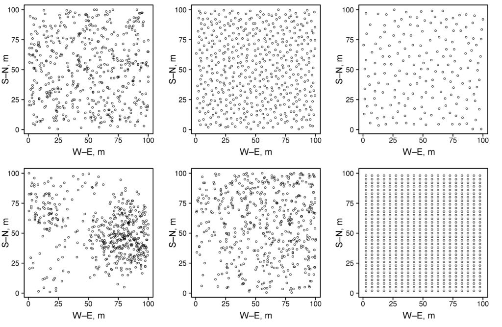
Figure 11. Implementation of different variants of initial tree placement: 1 — uniform pseudorandom; 2 — pseudorandom with a threshold distance (stand density priority); 3 — pseudorandom with a threshold distance (minimum distance priority); 4 — clustered; 5 — gradient; 6 — regular
The β-distribution (Gupta, 2011) is used to simulate the heterogeneity of height and diameter values of individual trees. The range of height and diameter values is specified in the input parameters of the submodel by specifying average, minimum and maximum values of these parameters, which allows generating asymmetric distributions. It is also possible to specify the degree of correlation between height and diameter values for individual trees. The additional parameter allows user to specify the shape of the distribution (convex, concave, uniform). Submodel structure allows to simulate multi-species stands, where it is possible to set the ratio between species at a certain type of spatial structure or to combine stands of several species, each of which is characterized by its own features of spatial structure.
Unit step of the model system
Competition for mineral nitrogen in the soil
The competition submodel between trees for mineral nitrogen in the soil, described in detail previously (Shanin et al., 2015a), simulates the growth and development of root systems, taking into account their adaptation to spatial heterogeneity in soil resource distribution and competitive pressures from neighbors. Within each cell of the simulated site, the distribution of resources and root biomass is assumed to be homogeneous. The submodel is individual-based and spatially-explicit, i.e., it takes into account the relative position and characteristics of all competing trees in the stand, and the nutrition zone of each tree is represented as an array of cells.
The total area of each tree’s nutrition zone is calculated based on the average (lavg) and maximum (lmax) root spreading distance (m):
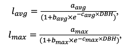
where DBH is the diameter of the tree trunk at breast height (cm), aavg, amax, bavg, bmax, cavg and cmax are empirical coefficients. Since root spreading distance decreases with increasing soil fertility and moisture, these parameters are modified depending on habitat conditions such as moisture and trophicity (additional multipliers mfert and mmoist). The area occupied by the root system is calculated based on the average root spreading distance as the area of a circle with radius equal to lavg.
To determine the conditions for including a cell (x,y) in the tree nutrition zone, the parameter px,y is used, which depends on the following: the amount of nitrogen in plant-available forms (kg m−2, is an output variable of the soil organic matter dynamics submodel) in a given cell (nx, y); the distance between the center of the cell and the base of the focal tree trunk (dx,y); and the root mass of other competing trees (kg m−2, is an output variable of the sub-model of production and organ biomass distribution) in the cell (mx,y):
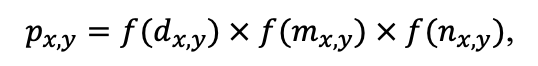 where the values of the corresponding variables are standardized to bring them to the range [0; 1]. Since the preference dependence of cell inclusion in the tree nutrition zone on the distance to the focal tree trunk and on the root biomass of competing trees decreases along with the growth of the index, an additional inversion of the standardized values is performed (1 − f(x)):
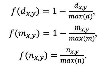
The parameter px,y is calculated separately for each tree. The calculation is done for all cells that are inside the potential root nutrition zone (circle with radius lmax) but are not yet included in the actual zone. The cells are then included in the nutrition zone according to the value of the px,y parameter.
The biomass of fine roots of a tree is distributed over the cells of the nutrition zone in proportion to the sum of values in a given cell that are f(mx,y) and f(nx,y), the biomass of skeletal roots is distributed in proportion to values of f(dx,y). The vertical distribution of root biomass of each tree between forest floor and mineral soil is described as follows:
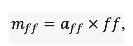
where mff is the fraction of total root biomass (separately for fine and skeletal roots) in a given cell that is in the forest floor; ff is forest floor thickness (cm), aff is a species-specific coefficient (also differs for skeletal (SRff) and fine (FRff) roots).
The aff coefficient has a species-specific modifier mstrat to account for the effect of changes in the vertical stratification of tree root biomass of different species when they grow together (Brassard et al., 2011; Shanin et al., 2015b). The parameters of vertical distribution of root biomass are calculated separately for each of the cells. The algorithm operation scheme is presented in Fig. 12.
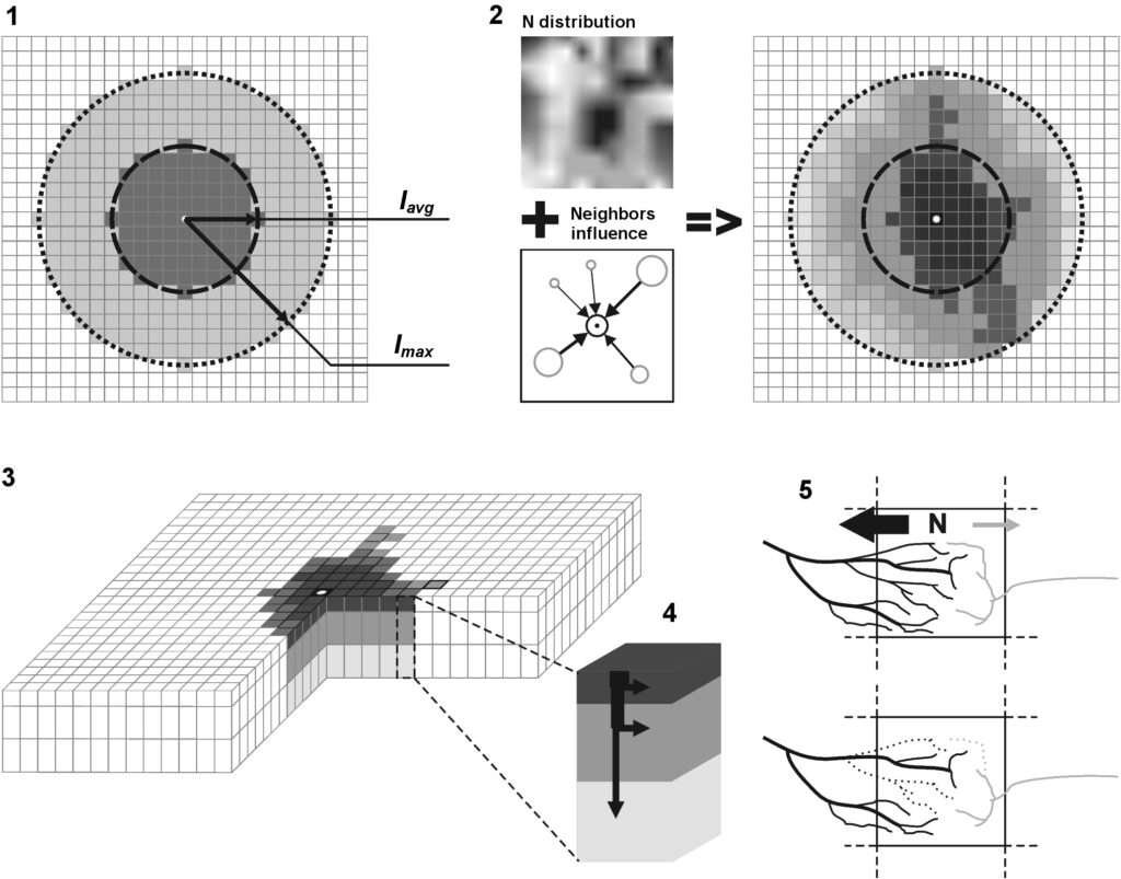
Figure 12. Block diagram of the annual step algorithm of the competition for available soil nitrogen submodel: 1 — calculation of the root nutrition zone area based on lavg (dark gray area) and determination of all cells that could potentially be included in the nutrition zone based on lmax (light gray area); 2 — calculation of the preference parameter for each cell in the potential nutrition zone, taking into account the heterogeneity of resource distribution and competitive pressure from neighboring trees; 3 — inclusion of cells in the root nutrition zone, with fine root biomass distributed among cells according to px,y values; 4 — calculation of vertical distribution of root biomass in each cell; 5 — calculation of N uptake in plant-available forms according to the fine root biomass of each competing tree. Reproduced from Shanin et al. (2015a)
Nutrient uptake is modeled independently for each cell. Available nitrogen is assumed to be distributed among competing trees in proportion to the ratio of their fine root biomasses in a given cell (Pagès et al., 2000; Schiffers et al., 2011), with an additional age-dependent modifier (Lebedev, 2012a; Lebedev, Lebedev, 2012):
where A is tree age (years), and aur, bur are species-specific empirical coefficients. Under the assumptions made, all of the nitrogen available to the trees is completely absorbed from the cell in a unit time step.
Competition for photosynthetically active radiation
The submodel of competition between trees for PAR was described in details previously (Shanin et al., 2020). Similar to the competition submodel for soil resources, it is individual-based and spatially-explicit, i.e., it takes into account the relative position and characteristics of all competing trees in a stand. The simulated area is divided into three-dimensional cells represented as rectangular prisms with the base size equal to the size of the simulation grid cell. The height of the cells is also set in the submodel settings. The crowns of all trees are approximated by such cells, each cell can contain the crown of only one tree. The submodel requires the following inputs: spatial location, species, age, height, and trunk diameter at breast height for each individual tree. The outputs of the submodel are the amount of PAR absorbed by each tree and the spatial distribution of PAR intensity under the canopy. The submodel is dynamic and able to reproduce changes in the crown shape of individual trees over time as a result of competition.
Crown size is determined by (a) the total height of the tree, (b) the height of the crown base, and (c) the maximum width of the crown. The crown is represented by one of the axisymmetric bodies such as cylinder, vertically asymmetric ellipsoid, semi-ellipsoid, cylinder, composite cone and inverted cone. Crown shapes are based on the basic shapes presented in some previous studies (e.g., Pretzsch et al., 2002; Widlowski et al., 2003), with additional modifications (Fig. 13).
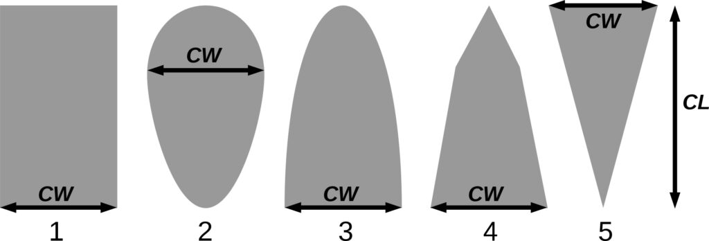
Figure 13. Flat figures forming axisymmetric bodies to represent species-specific crown shapes: 1 — cylinder, 2 — vertically asymmetric ellipsoid, 3 — semi-ellipsoid, 4 — composite cone, 5 — inverted cone. CW is the crown width at its widest part (i.e. doubled maximum crown radius), CL is the crown length in the vertical direction (total tree height minus crown base height). Reproduced from Shanin et al. (2020)
The equation for calculating potential crown radius uses trunk diameter at breast height (DBH) as predictor. The equation for calculating actual crown extent in the vertical direction uses tree height (H) and local competition indices as predictors (Thorpe et al., 2010) is as follows:
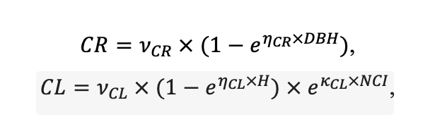
where CR is the crown radius at its widest part, CL is the crown length in the vertical direction, NCI is the competition index representing the local stand density around a given tree (see below), ν, η and κ are empirical coefficients (the CR index corresponds to the coefficients for crown radius and the CL index to the crown length). Thus, the intensity of competition (expressed through local stand density around the focal tree) affects crown size. Crown length is considered as the total height of the tree minus the height of the crown base.
When calculating competition indices, the influence of all trees (j = 1 … n) of different species (i = 1 … s), located no further than 10 m from the focal tree was taken into account. The submodel accounts for the decrease in competitive pressure from neighbors as the size of the focal tree increases:
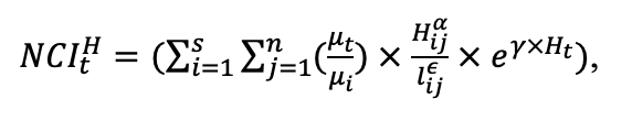
where lij is the distance between the focal and competing tree, Hij is the total height of the competing tree, Ht is the total height of the focal tree t; α, ε, γ, μ are species-specific empirical coefficients (Thorpe et al., 2010).
The obtained three-dimensional objects describing the shape and size of crowns of individual trees are divided into horizontal layers with 1 m intervals. If the crown does not occupy the entire layer vertically (which is possible for the bottom and upper of the layers on which the crown falls), the approximation submodel assumes that the crown is represented in a given layer if it occupies more than half the height of the layer. To avoid cases where the crown is not represented in any layer, for trees with crowns occupying less than half of any layer in the vertical direction, the submodel assumes that the crown is represented in the layer in which its extension in the vertical direction is maximized. The radius of the crown in each layer is calculated as the radius of an axisymmetric body representing the basic shape of the crown at the relative height corresponding to the midpoint of that layer. Within the layer, the crown is approximated by rectangular prisms.
To modify crown radius due to competitive pressure from neighboring trees, the areas potentially occupied by its crown must be identified for each tree. This step involves partitioning the simulated site into subsets of cells, where each subset meets the following two conditions: (a) it is closer to a given tree than to other trees, which is done by implementing Voronoi partitioning (Tran et al., 2009) in discrete space, and (b) the number of cells occupied by the tree crown in a given layer does not exceed the potential crown projection area (numerically equal to the area of a circle with radius equal to the radius of the crown in a given layer). Such subsets are constructed separately for each layer, and only those trees with crowns represented in a given layer are considered for partitioning.
In the next step, the submodel simulates the distribution of biomass of photosynthetic (leaves or needles) and non-photosynthetic (trunk and branches) organs between the cells that make up the crown of the tree. The biomasses of different tree organs are output parameters of the production and biomass distribution submodels (Shanin et al., 2019). The submodel accounts for heterogeneity in both vertical and horizontal (from trunk to crown periphery and in different directions) biomass distribution between cells, while biomass distribution within a cell is assumed to be homogeneous. The submodel is based on the assumption that the spatial asymmetry in the distribution of photosynthetic organs within the crown is determined predominantly by competition from neighboring trees. The vertical distribution of biomass within the crown is described as follows:
where mcum is the accumulated relative mass of a crown component (photosynthetic or non-photosynthetic organs) in a given cell, Hrel is the relative height of a given point within the crown (taking the total crown length as 1), and σ, τ, ψ, ω are empirical coefficients (Tahvanainen, Forss, 2008). Scaling is then applied to set mcum equal to 1 with Hrel equal to 1. The vertical distribution of trunk biomass is calculated based on its representation as a truncated cone, strictly circular in any horizontal section, with the radius of the upper circle equal to 0.25 of the base radius. The trunk biomass in each layer is added to the branch biomass for the cell whose horizontal coordinates coincide with those of the trunk base. According to the algorithm, biomass distribution over the horizontal crown layers of each tree is first made and then biomass distribution between cells within a given layer is calculated.
Since detailed data on the radial distribution of phytomass are not available, the description of the radial distribution of biomass within a crown is based on the assumption that the biomass of photosynthetic organs increases linearly from the crown center to the periphery and from the northern to southern part of an individual crown (Olchev et al., 2009; Bayer et al., 2018). The construction of the actual crown shape is shown schematically in Figure 14.
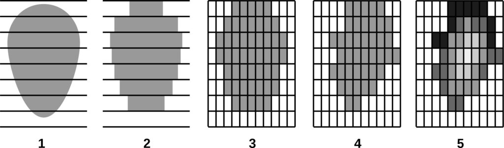
Figure 14. Schematic representation of the algorithm for constructing the actual crown shape (a vertical section of the crown, not passing through the trunk, is taken as an example): 1 — basic crown shape; 2 — division of the crown into horizontal layers; 3 — approximation of the crown by three-dimensional cells; 4 — modification of the crown shape in the horizontal direction in accordance with asymmetric competitive pressure from neighboring trees; 5 — distribution of aboveground biomass between cells. Reproduced from Shanin et al. (2020)
Input and absorption of photosynthetically active radiation (PAR) in each cell (x,y,z) is calculated as the sum of direct and diffuse PAR values, in turn calculated as products of their daily sums above the canopy on a given day by the corresponding values of relative values (coefficients) of transmittance and/or absorption for each cell:
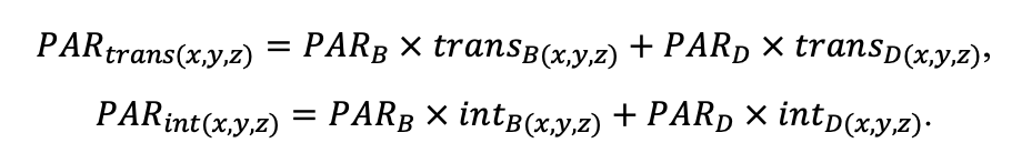
The incoming solar radiation above the canopy is calculated from the trajectory of the Sun’s apparent motion across the sky, as well as from cloud cover, which in this version of the submodel is indirectly accounted for through the 24-hour air temperature range. The necessary astronomical calculations are performed according to Strous (2022).
The altitude hʘ and azimuth ψʘ of the Sun are calculated from the dependencies:
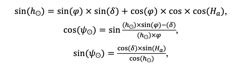
and the daylight hours are calculated as
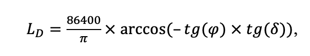
where φ is the latitude, Ha is the hour angle (time relative to true noon expressed in radians), δ is the declination of the Sun (depending on the ordinal number of the day of the year d):
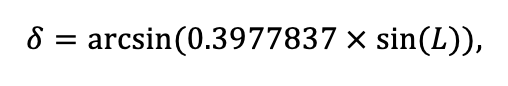
where L is the ecliptic longitude:

M is the average orbit anomaly:
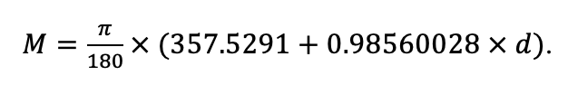
The extraatmospheric integral solar radiation coming to the surface perpendicular to the rays is calculated by the following equation:
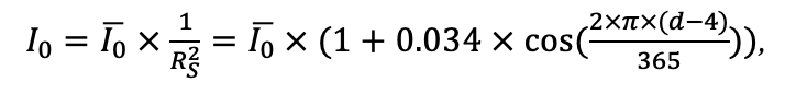
where ![]() =1367 W m−2 is the solar constant, is the distance from the Earth to the Sun (a. e.), and d is the ordinal number of the day of the year. The extraatmospheric insolation on a horizontal surface is accordingly calculated as
=1367 W m−2 is the solar constant, is the distance from the Earth to the Sun (a. e.), and d is the ordinal number of the day of the year. The extraatmospheric insolation on a horizontal surface is accordingly calculated as
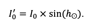
The corresponding daily amount is calculated as
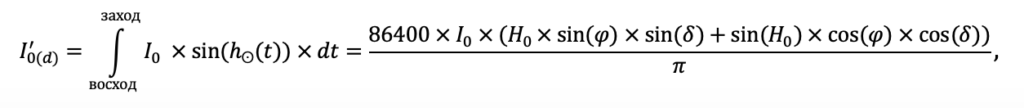
where Н0 is the hourly angle of sunset.
Extraatmospheric PAR fluxes are calculated in a similar way, using the corresponding value for PAR instead of the integral solar constant:
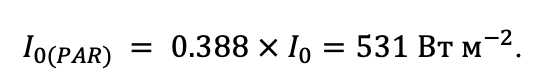
The total integral solar radiation under actual cloudy conditions is calculated from the extraatmospheric insolation and the daily range of air temperature change (ΔT = Tmax − Tmin), which is used as an indirect characteristic of cloudy conditions (Bristow, Campbell, 1984):
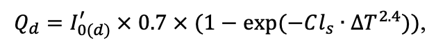
where the coefficient Cls = 0.004 is for warm season and 0.010 is for cold season.
Next, to estimate PAR fluxes, daily sums of total PAR are calculated from the sum of integral total radiation and its relation to the value of extraatmospheric insolation using a data-driven relationship (Yu et al., 2015):
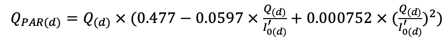
To divide the total PAR into direct S’PAR and scattered DPAR, we use the dependence of the relative fraction of scattered PAR in the total PAR (kdp) on the ratio of the actual total PAR to the corresponding extraatmospheric value (ktp = QPAR(d) / I’PAR(d)), approximated by us based on data from Jakovides et al. (2010):
kdp= 0.6182+ 0.3397×cos(3.9468×ktp -0.2469).
Hence:
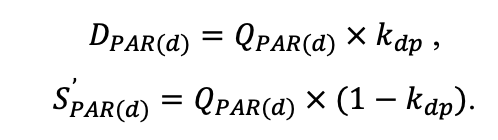
.
Assuming a direction-independent (isotropic) input of diffuse radiation over the canopy, the spherical exposure to diffuse radiation is equal to twice its flux to the horizontal surface (van der Hage, 1993):
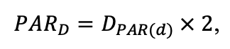
and spherical irradiance of a straight PAR is equal to its flux on the perpendicular surface and is estimated from the following relation:
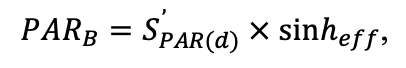 where sin(heff) = S’d / Sd is the ratio of daily sums of direct radiation on horizontal and perpendicular to solar rays surfaces (daily weighted average or “effective” sine of the Sun’s height), the relationship of which with the Sun’s height at noon hʘmax is estimated by us from the data of the Applied Scientific Reference Book on Climate of the USSR (1988–2002) for 32 stations of the forest zone of the European part of Russia:

where

Relative values (coefficients) of transmittance and absorption of the PAR, averaged over the directions of incoming radiation, are calculated for each cell. For scattered radiation it is twice a year (for the vegetation period and for the cold season, taking into account the presence/absence of foliage of deciduous species), for direct radiation it is based on the trajectory of the visible motion of the Sun across the sky for the middle of each month.
The directions of the calculated scattered radiation rays are calculated using the Fibonacci lattice algorithm (Stanley, 1988) in order to distribute them uniformly over the celestial hemisphere. Under the assumption of isotropy, the fraction of scattered radiation energy attributable to each of the n calculated directions and equals to 1 / n.
Direct radiation ray paths for calculation of relative transmittance (absorption) values are set at 1-hour intervals. The energy distribution by directions is set in proportion to the share of the corresponding hourly sums in the daily sum of the direct PAR to the surface perpendicular to the rays.
For this purpose, the direct integral radiation to the perpendicular surface under clear sky is calculated as a function of the Sun’s altitude and the atmospheric transparency coefficient P2 (Evnevich, Savikovsky, 1989):
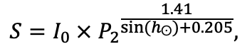
and then taking into account the relative fraction of PAR in the integral direct radiation (Mõttus et al., 2001),
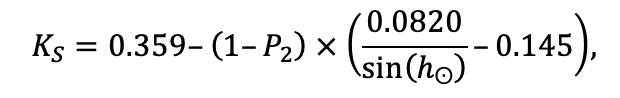
the direct PAR is calculated:

The corresponding daily amount is calculated as follows
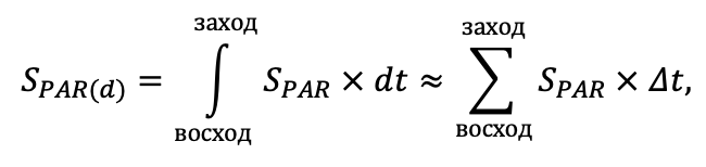
where Δt = 3600 s. The fractions in it, falling on each i of the calculated directions, are respectively as follows:
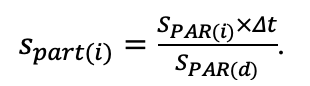
The calculation of relative radiation transmittance for each direction i in each layer z is calculated from the path length of the i beam in the layer Δli = 1 / sin(hi) and the radiation absorption coefficients k(x,y,z) in the input and output cells crossed by the beam in a given layer. Absorption coefficients are calculated from the sum of relative leaf area (LAD — Leaf Area Density) and non-photosynthetic phytoelements (WAD —Wood Area Density) represented in a given cell. In the most elementary case (under the assumption of random placement of phytoelements within the cell and their uniform orientation along the directions) there is the following:
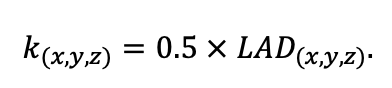
The attenuation of the i ray in layer z is calculated as the exponent of the product of the attenuation coefficients over the length of the ray in the layer, and the total attenuation of the ray reaching the cell (x,y,z), aT(i,x,y,z), is equal to the product of the transmission coefficients of all layers traversed by the ray.
The transmittance factor for the corresponding component of spherical irradiance is calculated as a weighted average of all directions, taking into account their share in the daily sums of PAR reaching the upper boundary of the canopy. Thus:
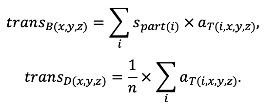
The relative absorption by foliage in a cell is respectively calculated from the radiation reaching the cell and k(LAD) in the cell. If k(x,y,z) is direction-independent (uniform leaf orientation), the PAR absorption by the foliage in the cell is proportional to the spherical irradiance:
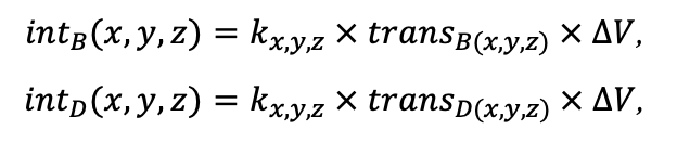
where ΔV is cell volume.
Radiation input to the soil surface (ground cover) is calculated in terms of flux density per horizontal (or inclined in case if microrelief is taken into account) surface, considering the slope of rays and their attenuation. In particular, for a horizontal surface, all transmittance values of individual rays are multiplied by the corresponding sin(hi) value before summing.
The amount of absorbed PAR in quantum terms (uAPAR) is calculated accounting for the quantum equivalent of PAR, taken to be 4.56 mol MJ−1 (Mõttus et al., 2013).
Tree biomass production
The productivity submodel detailed in the previous study (Shanin et al., 2019) is based on the algorithms of the well-known 3‑PG model (Landsberg, Waring, 1997; Seidl et al., 2012). This submodel provides a simplified reproduction of basic ecophysiological processes and allows us to calculate the biomass production of an individual tree depending on the number of resources it receives and on the tree’s response to changes in external conditions.
Potential gross primary production (calculated in kilograms of absolutely dry mass per tree) based on the PAR intercepted by a tree is calculated in daily time steps as follows:
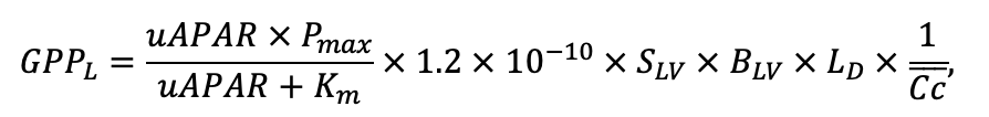
where uAPAR is the PAR absorbed by the tree (μmol m−2 s−1, which is calculated in the crown competition submodel); Pmax is species-specific maximum photosynthesis intensity in terms of carbon, μmol m−2 s−1; Km is the PAR intensity at which 0.5 of the full photosynthetic intensity is reached, μmol m−2 s−1; 1.2 × 10⁻¹⁰ is the conversion coefficient from μmol to kg of carbon; SLV is specific one-sided leaf surface area, m2 kg−1; BLV is total biomass of tree foliage, kg (used to go from 1 m2 of leaf area to total leaf area of the tree); LD is daylight hours, s, ![]() is the weighted average carbon concentration across all fractions of tree biomass.
is the weighted average carbon concentration across all fractions of tree biomass.
An air temperature-dependent modifier (Mäkelä et al., 2004) is calculated in daily time steps (d) based on a first-order delay model. The first stage calculates TE, a “smoothed” temperature that takes into account the inertia of temperature acclimatization and is calculated based on the average daily air temperature for the current (d) and preceding (d−1) day:
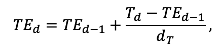
where dT is a biome-specific constant determining the delay time (in days) of response to temperature change (Mäkelä et al., 2008). Td is the average daily air temperature.
Temperature acclimation state TA is derived based on the threshold (biological minimum of photosynthesis) temperature T0:
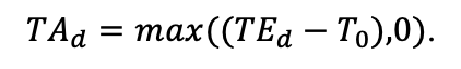
The final value of the temperature-dependent modifier fT is calculated with respect to the saturation level temperature T1. Moreover, the parameter T2 was added to the modifier calculation procedure to take into account the decrease in productivity when the temperature rises above the threshold level:
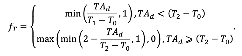
Thus, T0 is the temperature at which the production process stops, T1 is the temperature corresponding to the saturation point, above which there is no increase in productivity, and T2 is the temperature at which suppression of production processes begins due to heat stress.
The productivity response associated with VPD (vapor pressure deficit) is based on a function similar in purpose to that used in the ecological-physiological model of M.D. Korzukhin and Y.L. Celniker (Korzukhin et al., 2004, 2008; Celniker et al., 2007, 2010; Korzukhin, Celniker, 2009, 2010). This modifier is calculated as follows:
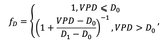
where VPD is vapor pressure deficit (kPa); D0, D1 are empirical parameters (D0 corresponds to the value of VPD, up to which its increase does not lead to conductivity decrease, and D1 corresponds to the value of VPD, at which the stomatal conductivity decreases twice).
A modifier of the productivity response as a function of soil moisture availability is calculated from the soil moisture potential ψ (Hanson et al., 2001; Wullschleger, Hanson, 2003). It is a linear function of ψ ranging from the lowest field moisture capacity ψfc to the species-specific ψmin:
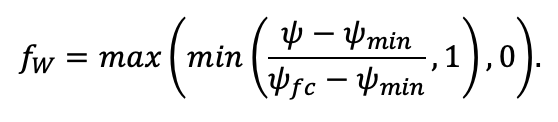
The dependence of PAR utilization efficiency on CO2 concentration is calculated as follows
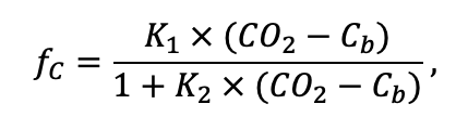
where
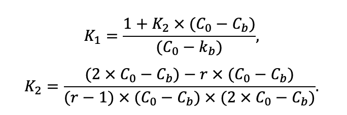
Here CO2 and C0 are the current and baseline CO2 concentrations, respectively. Cb corresponds to the photosynthesis compensation point and is equal to 80 ppm (Coops et al., 2005).
PAR interception for deciduous species is limited by the length of the growing season, which is determined by the value of the vegetative index GSI. For its calculation such parameters as duration of photoperiod L, minimum daily temperature Tmin and vapor pressure deficit (VPD) were used.
The effect of productivity decline during tree senescence (fA) is calculated as follows (Räim et al., 2012):
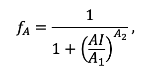
where A1 and A2 are empirical coefficients and AI is calculated as:
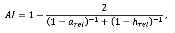
where relative age arel and relative height hrel are calculated as the ratio of tree age and height to the corresponding species-specific maxima (Amax, Hmax) and are indicators of senescence.
The dependence of productivity on the amount of nitrogen consumed by the tree (fN) is calculated based on the value of maximum theoretical nitrogen consumption by the tree (per 1 kg of growth):

where Ni is the specific nitrogen consumption by different tree organs, in kg of nitrogen per 1 kg of biomass growth of an organ, BPi is the share of growth of a given organ in the total biomass growth (see below), where i corresponds to the indices of different tree organs (ST — trunk, BR — branches, LV — foliage or needles, SR — skeletal roots, FR — fine roots).
Potential productivity as a function of the amount of available N is calculated from the amount (kg) of N consumed by the tree from the soil (Nuptake), which is calculated in the root competition submodel; the amount of buffer N stored by the tree is also taken into account:
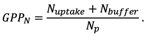
The value of the modifier fN is calculated based on the ratio of potential growth depending on the amount of available N and potential growth limited by other factors. The value of the modifier is bounded from above by the value 1, thus characterizing the saturation output of the function:
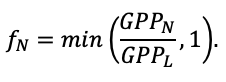
The efficiency of γeff resource utilization (Seidl et al., 2005; Swenson et al., 2005) depends on modifiers related to environmental conditions and physiological characteristics of the tree:

where an empirically chosen value of the coefficient w (Frolov et al., 2020a) determines the balance between the two methods of evaluating the interaction between modifiers.
Actual gross primary production is calculated as follows:
![]()
Excess absorbed nitrogen is stored in the form of a buffer stock. The submodel also accounts for the movement of some N from dying leaves/needles (LITLV) to the N buffer before they fall:

where NLIT is nitrogen content in leaf/needle litter, LITLV is mass of annual leaf/needle litter.
Respiration in terms of carbon (C‑CO2) is calculated in daily increments and consists of two components. Maintenance respiration is calculated as
![]()
where BLV, BFR, BST, BBR, BSR are the biomass of leaves/needles, fine roots, trunk, branches and skeletal roots, respectively, CLV, CFR, CST, CBR, CSR are the carbon content of leaves/needles, fine roots, trunk, branches and skeletal roots as a fraction of the absolute dry mass, and Q10 is calculated as:
![]()
where Td is the average daily air temperature (Wang et al., 2011).
The second component (growth respiration) is calculated as a constant fraction of gross primary production (Jiao et al., 2022):
![]()
Net primary production equals gross primary production minus respiration costs:
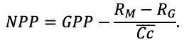
If the value of fN is less than 1, the excess assimilates are converted to the amount of root exudates:
Tree leaf stomatal conductance is calculated considering photosynthetic rate, relative humidity (rh), and leaf surface CO2 concentration (Cs) using the following formula (Pace et al., 2021):
where Kbb is the Ball-Berry coefficient (dimensionless), GPP is the gross primary production (in terms of carbon, μmol m−2 s−1), CO2 is the volume concentration of CO2 (μmol mol−1), and gs0 is the minimum value of the stomatal conductance (mol m−2 s−1).
According to Zhu et al. (2011), tree transpiration (ET, kg m−2 s−1) is calculated as
where gsW is the stomatal conductance of H2O equal to (gs / 1.6), VPD is the vapor pressure deficit between the intercellular space and the air layer directly above the leaf surface (taken equal to the VPD of atmospheric air assuming saturating humidity of air in the intercellular space and equality of leaf and ambient air temperatures), Patm is the atmospheric pressure taken constant and equal to 105 Pa, and μW is the molar mass of water (g mol−1).
Biomass allocation and spatial distribution of litter
The rank distribution equation, described in more detail in previous studies (Komarov et al., 2017b; Shanin et al., 2019), is used to describe the distribution of biomass growth among tree organs. In the case of tree biomass, rank characterizes the place of the corresponding tree organ in a row ordered by decreasing amount of resource input. Accordingly, this allocation allows us to calculate the amount of resource delivered to each organ in the tree, using the predetermined rank of that organ as a predictor:
where i is the fraction rank (1 — trunk, including bark; 2 — skeletal roots; 3 — branches; 4 — foliage or needles; 5 — fine roots), BPi is the fraction of the i-th fraction in the total tree mass, a and b are empirical coefficients (Isaev et al, 2007; Komarov et al., 2017b). The values of them are calculated on the basis of tree trunk diameter at breast height (DBH) and empirical coefficients (crank, drank, erank, frank). The procedure for calculating biomass distribution across fractions also takes into account the influence of habitat conditions (Thurm et al., 2017; Weemstra et al., 2017).
When the submodel is initialized, the absolute mass of all fractions is calculated based on the allometric equation for BST (trunk biomass), for which the estimates are the most accurate (due to the large number of observations and large values of the measured quantity):
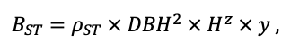
where ρST is species-specific trunk mass in absolutely dry state (including bark), kg m−3; DBH is tree trunk diameter at breast height, m; H is tree height, m; and z, y are empirical coefficients. After calculating the trunk mass, the total mass of the tree is determined based on the previously calculated trunk fraction. From this, the masses of all organs are further calculated.
The submodel also calculates annual litter (as a fixed biomass share of each biomass fraction) and calculates the net biomass growth of each fraction (total growth excluding annual litter). If the net increase in total biomass takes a negative value, the tree is considered to be dying off (deterministic mortality component). Based on the estimated trunk biomass increment, the height and diameter increment of the trunk are calculated.
In addition to the above-described deterministic component of tree mortality based on net biomass growth, the submodel implements a stochastic component (Seidl et al., 2012). It is based on the increasing probability of tree mortality as its age A (years) approaches the species-specific maximum value Amax:
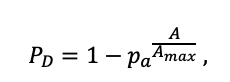
where pa is the share of trees reaching the maximum age.
The spatial distribution procedure for needle/leaf litter of the tree stand calculates the mass of leaf or needle litter entering each cell of the simulation grid. For each tree, we calculate the spatial distribution of litter (D) in cells with (x,y) coordinates, which is determined by the average radius of the tree crown F (CR, calculated in the PAR competition submodel) in its widest part. The radius of the dispersal zone is defined as a species-specific fraction of tree height (DLIT parameter):
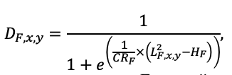
where L is the distance from the crown mass center of the tree F to the cell with coordinates (x,y). To account for the influence of microrelief, the spatial distribution of litter is adjusted for the relative height of the cell (MR) with (x,y) coordinates:
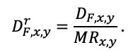
The litter mass of the tree F falling down to the cell with coordinates (x,y) is calculated as
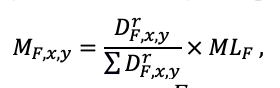
where MLF is the mass of needle/leaf litter of the tree F.
To account for the influence of crown asymmetry of each tree on the spatial distribution of litter, the tree crown mass center is taken as the center of the spreading zone, which is calculated as the weighted average coordinates (x,y). The total needle/leaf mass in cell (x,y) along the vertical profile is used as weights.
Branch litter is assumed to fall evenly into all cells overlapped by the crown projection of a particular tree. The distribution of skeletal and fine root litter is calculated in the root competition submodel based on the modeled structure of root systems and estimated root die-off rates. Until the improved procedure is finalized, the spatial distribution of trunk wood and bark litter is assumed to be similar to that of branch litter.
Living ground cover
The eco-CAMPUS submodel, which is a modified version of the CAMPUS-S model (Frolov et al., 2020a, 2020b), was developed to model the contribution of living ground cover plants to carbon, nitrogen balance and forest ecosystem dynamics. The eco-CAMPUS submodel, integrated into the overall model system, is a customized process-based simulation model with a space represented as a three-dimensional grid. The submodel combines several modeling techniques such as cell-automation (state of a cell depends on the state of its neighbors) and L‑systems technique (modular evolution of a clone system). Unlike the СAMPUS-S model, in which no more than one plant can be presented in one cell, eco-CAMPUS allows the presence in one cell of several plants of the same or different species occupying different height layers (the submodel structure has 6 layers: 0–10, 10–20, 20–30, 30–40, 40–50 and 50–100 cm). In this case, one plant can occupy more than one cell according to the morphological structure that changes during the life cycle. Since the submodel is designed to analyze the population dynamics of both clonal and non-clonal plants, the term “plant unit” (PU) is used in the modeling to denote an elementary accounting unit. This unit represents either a partial formation within a clonal plant (i.e., a shoot together with a rhizome) or a single individual of a non-clonal plant. The development of plants in time is accounted for in the submodel through their ontogenetic states (Evstigneev, Korotkov, 2016). For each of the ontogenetic states (OS), the corresponding projection area of the aboveground and belowground parts, the height of the aboveground part of the plant, and the height of attachment of photosynthetic organs are given. Each ontogenetic state has a different duration and all transitions are probabilistic. The time step of the submodel is 1 day.
In the initialization step, a set of PUs from a given list of species is placed in each cell. The ratio of PUs in a cell and their total projective coverage (proportion of occupied area in a cell) is determined by the coefficient of optimality of conditions (generalized response of productivity to a complex of environmental factors). The ontogenetic states and absolute ages of PUs are set probabilistically given the initial ontogenetic spectrum, which is the input parameter.
A unit step of a submodel consists of several sequentially executed operations. The age increase occurs daily for each PU. In this case, both absolute and relative age (duration of PU stay in the current OS) increase by the value inverse to the duration of the vegetation period. The use of growing season fractions instead of calendar days makes it possible to model the population dynamics of species with a wide geographical range growing at different latitudes. When PU reaches a relative age equal to the duration of the current ontogenetic stage, the transition of PU to another ontogenetic stage is calculated probabilistically. The probability of successive transition to the next stage of ontogenesis (Ptr) is considered to be equal to the ratio of potential growth (growth in optimal conditions during the period of stay in the current OS) to actual growth. The probability of PU death is calculated as (1 − Ptr). In case of change of ontogenetic state, the diameter, height of PU (occupied layer) and height of attachment of photosynthetic organs, as well as the maximum radius of the root nutrition zone changes. PU leaf area is calculated as multiplication of biomass and specific leaf area. The relative PU leaf area (LADFGV) is calculated as the ratio of the PU leaf area to the projection area of its photosynthetic organs and distributed among the PU-occupied layers. The submodel does not explicitly represent the location of individual PU within the cell. Therefore, as the size of the shoot system increases, the fraction occupied by PU in the current cell or in one of the neighboring cells increases as well. The probability in which cell the fraction of a given PU will increase is directly proportional to the coefficient of conditions optimality and inversely proportional to the projective cover in the cell. The number of seeds in the modeled area is calculated as the product of the PUs number in the generative OS of each species and the species-specific number of seeds per PU. It distributes among cells randomly once per growing season (when the maximum proportion of generative organs in total biomass is reached).
The calculation of PU biomass production takes into account the same factors and resources used in the stand biomass production submodel. Competition for light between PUs in the cell is realized based on the assumption that light rays passed under the canopy are oriented predominantly vertically and consistently pass through all layers of living ground cover. The attenuation of their intensity is exponential. The PAR attenuation coefficient at each layer is calculated using the following methodology (Campbell, 1986). For each PU, the leaf orientation coefficient (Xi) is calculated as the ratio of the length of the horizontal to the length of the vertical projection of photosynthetic organs, which is used to calculate the PAR attenuation coefficient (![]() ):
):
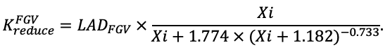
The PAR attenuation in the cell at each layer is calculated as the exponent of the product sum of the PAR attenuation coefficients of all PUs represented in a given layer of the cell by the ray path length in the layer. PAR captured in the layer is calculated as the difference of the PAR flux densities at the upper and lower boundaries and distributed among the PUs present in the layer in proportion to their PAR attenuation coefficients. Competition for available nitrogen and available soil moisture, as well as the calculation of biomass production, occurs according to algorithms similar to those for trees (described in the respective subsections). In the vegetative period, the distribution of biomass between PU organs is uneven. From the point when all PU organs (leaves, vegetative shoots, generative shoots, rhizomes and fine roots) are fully developed, the rank distribution equation is used to describe the distribution of biomass growth (Frolov et al., 2022). Up to this point, biomass growth is distributed among those organs with shares of total biomass lower than those determined by the rank distribution. If PU is in generative OS, the biomass of vegetative organs grows first, and only after they reach the necessary share in the total biomass the growth of generative organs begins. Leaf and shoot litter occurs on the last day of the growing season, fine root litter occurs daily, and rhizomes die off only with PU. The fraction of the organ mass reaching the litter is the submodel input parameter. Before the photosynthetic organs in perennial plants fall, nitrogen resorption is performed with its addition to the organ with maximum biomass.
Vegetation water regime and soil hydrothermal regime
A simple balance approach was used for modeling soil moisture. Obviously, the change in moisture content of the active soil layer ΔW = W2 − W1 can be assumed to be equal to
![]()
where r is precipitation, E is evapotranspiration (gross evaporation), f is runoff, W1 and W2 are moisture stocks at the beginning and end of the modeling step.
When modeling processes related to the spatial heterogeneity of ecological conditions in the forest, the most appropriate is a differentiated approach to the consideration of evaporation by different forest elements, which makes it possible to take into account their influence on moisture dynamics. In this case, evapotranspiration is represented as a sum of three summands (Fedorov, 1977):
![]()
where Et is stand transpiration; Ei is evaporation of precipitation retained in the forest canopy; and Es is evaporation from the ground cover.
The amount of water ETS withdrawn from a soil cell with coordinates (x,y,z) during transpiration is calculated considering the spatial distribution of fine tree root biomass mFR(x,y,z,n):
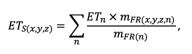
where
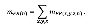
The amount of water ETC(x,y,z,) released by leaves during transpiration is calculated considering the spatial distribution of tree leaf biomass mLV(x,y,z,n):
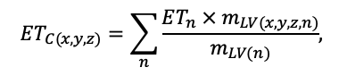
where
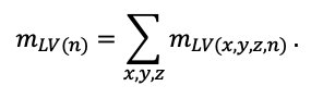
Potential evapotranspiration PET is calculated using the following relationship:
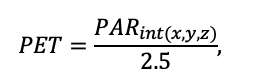
where 2.5 MJ kg−1 is the specific heat of evaporation of water.
Calculation of the total area of foliage and tree branches per canopy projection cell is performed by the following formula
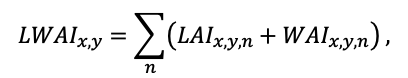
where LAI is leaf area index, WAI is branch area index (m2 m−2).
Based on LWAI, the water-holding capacity of crowns CSCx,y is calculated (Dickinson, 1984):
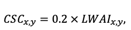
The amount of precipitation retained by the forest canopy is determined using the expression proposed by Y. V. Karpechko (1997):
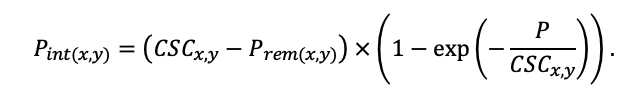
The actual canopy water content Pcurr(x,y) is calculated as the sum of intercepted precipitation, water remaining from the previous step Prem(x,y), and water released by transpiration (or guttation):
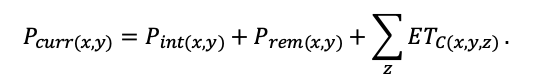
Canopy evapotranspiration Estand(x,y) is calculated as the minimum value from potential evapotranspiration and canopy water content:
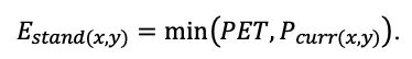
Water runoff from leaves and branches DripLV(x,y) is calculated as the difference of current canopy storage, evaporation from the canopy, and canopy capacity:

The amount of water remaining in the canopy for the next step, Prem, is calculated as
Water evaporation by ground cover is calculated from (Williams, Flanagan, 1996; Daikoku et al., 2008):
where WFF is the moisture reserve in litter, FCFF is its value at the lowest field water holding capacity.
The amount of precipitation that has passed under the canopy, Pbc(x,y), is calculated by the formula
Snow in the submodel is represented by the following three fractions: fresh (SWEf), frost-bound (SWEi), and melted (SWEw), the water supply of which is represented by water equivalent. The amount of precipitation that came in the solid phase Psol is calculated using the formula (Grossi et al., 2017):
where Th = +2 °C, Tl = 0 °C.
When calculating snow and ice melt, a modified method of temperature index calculation was used, which takes into account air temperature and incoming shortwave radiation (Rellissiotti et al., 2005):
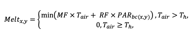
where MF = 1.2 mm day−1 °C−1, RF is 2.61 m2 mm MJ−1 (Rellissiotti et al., 2005). The submodel assumes that fresh snow is the first to melt:
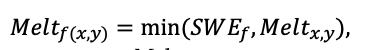
if its amount is less than Meltx,y, the ice starts to melt:
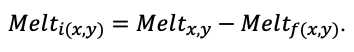
Freezing is considered using the classical temperature index method (Finsterwalder, 1887):
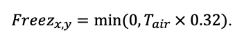
When the liquid water content of a snow layer exceeds its water-holding capacity, the excess water flows into the underlying layer. The water-holding capacity of snow WHC is calculated using the equation proposed by Pahaut (1975):
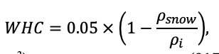
where ρsnow is the density of snow (kg m−3), ρi is the density of ice (917 kg m−3).
The amount of water that reaches the soil, liqflow(x,y), is calculated as

Water storage in fresh snow fraction (SWEf):
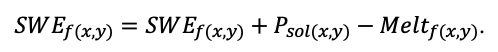
Water storage in ice fraction (SWEi):
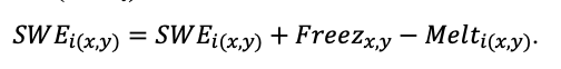
Water storage in liquid fraction (SWEw):

The density of falling snow (kg m−3) is calculated using the following equation (Parajuli et al., 2020):
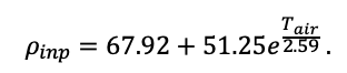
Fresh snow fraction density (kg m−3) is calculated by the following formula:
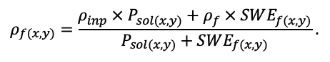
Total snow density (kg m−3) is calculated as
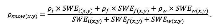
Snow cover height (m) is calculated as
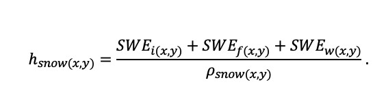
The thermal conductivity TCsnow(x,y), heat capacity HCsnow(x,y) and thermal diffusivity TDsnow(x,y) of snow are calculated using the following formulas (Yen, 1962, 1981):
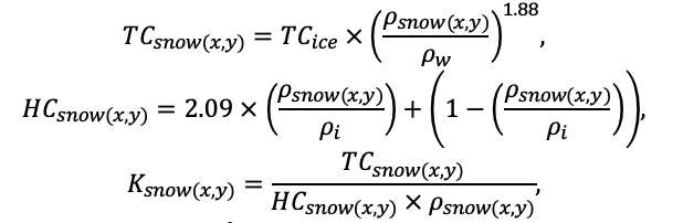
where ρw is water density (1000 kg m−3).
Soil organic matter concentration OMconc(x,y,z) is calculated as the ratio of the organic matter mass mOF(x,y,z) to the total soil mass in the cell:
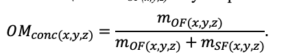
The density of the solid phase of the soil layer in the cell is calculated as
![]()
where 1.35 and 2.65 (g cm−3) are the density values of soil organic matter and mineral particles, respectively. The moisture content of stable wilting, WP and the lowest field capacity FC in the cell (x,y,z) are calculated according to the equations proposed by W. Balland et al. (2008) and converted to volumetric moisture units (m3 m−3):
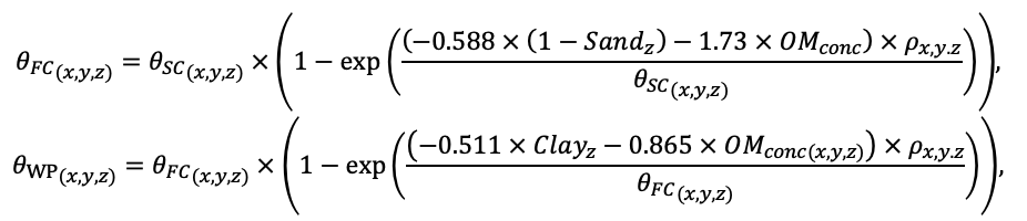
where Sand is the content of sand (particles > 0.05 mm), Clay is the content of clay (< 0.002 mm), in mass fractions (kg kg−1), and SC is the total water capacity (total porosity), m3 m−3:
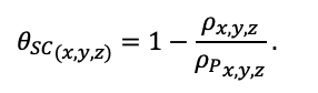
The corresponding values of moisture reserves in the layer Δz, accordingly, are equal to
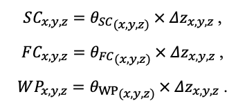
The saturated hydraulic conductivity HCsat(z) is calculated as follows (Campbell, 1985):

The unsaturated hydraulic conductivity HCx,y,z is calculated as follows (Campbell, 1974):
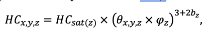
where θx,y,z represents soil moisture (m3 m−3), φ and b are coefficients calculated according to Cosby et al. (1984):
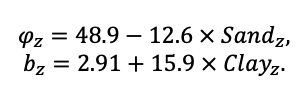
Since the unsaturated hydraulic conductivity in different cells of the soil profile can be heterogeneous and varies nonlinearly, the logarithmic mean of unsaturated hydraulic conductivities of neighboring cells is used to calculate moisture transport:
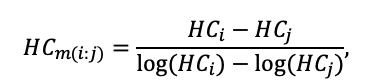
where HCi and HCj are unsaturated hydraulic conductivities of neighboring cells. Water storage in each soil layer is calculated sequentially from top to bottom in each step of the submodel. The amount of water flowing into the underlying soil layer is calculated using the following formula:
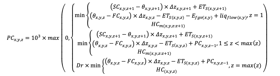
where Dr is considered equal to 1 for good and 0 is for poor drainage.
Moisture reserve in the soil layer is calculated using the following formula:
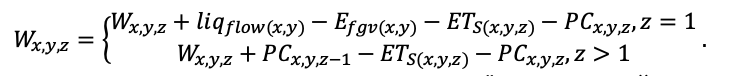
Potential water flows in each of the four directions in the horizontal plane (forward, backward, right and left) depend on the hydraulic gradient equal to the sine of the slope angle and are calculated as follows
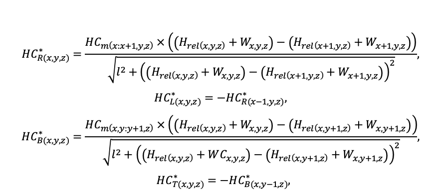
where Hrel is the relative cell height due to microrelief (m), and l is the horizontal dimension of the cell (m). Space is torus wrapped.
The sums of positive (HC+) and negative (HC−) fluxes are calculated for each cell (x,y,z):
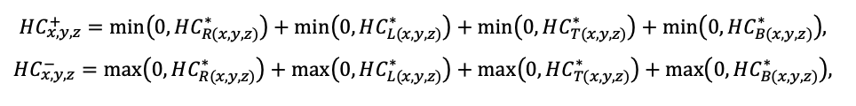
The weights of positive (outgoing) and negative (incoming) flows in a cell are calculated independently:
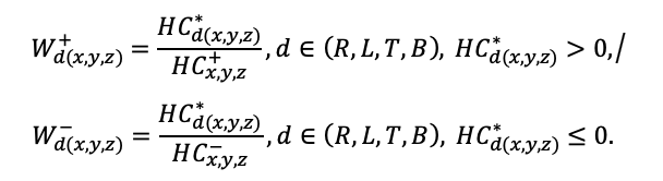
where d corresponds to the direction of each of the four flows. The limitation of positive flows is determined by the difference in cell water storage and field water capacity:

The limitation of negative flows is determined by the difference between total moisture capacity and water storage in the cell:

The resulting fluxes (PCR, PCL, PCT, PCB) are calculated as the smallest between the positive and complementary negative fluxes according to the module:
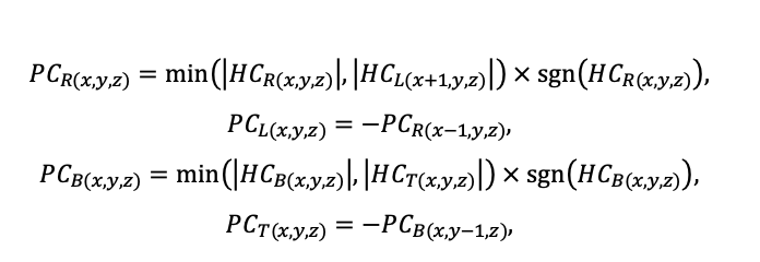
where sgn(HCdЄ(R,L,T,B)) is an indicator of HCdЄ(R,L,T,B)) flow sign (equal to +1 if the flow is positive and −1 if it is negative). Water storage in the cell after lateral transfer ( ) is calculated as the difference of water storage in the cell and flows in the four directions:

The volumetric moisture content of the soil layer in the cell is calculated as
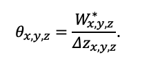
Soil temperature (Ts) affects most soil processes as well as plant growth. Together with chemical and physical characteristics of soil organic matter, soil temperature is one of the main variables controlling soil biological activity (e.g. Lundegårdh, 1927; Kätterer et al., 1998; Frank et al., 2002). Consequently, a spatially-explicit prediction of soil temperature dynamics is necessary for the application of other submodels such as the soil organic matter dynamics (SOM) submodel. Unfortunately, spatially-explicit soil temperature data are rarely available (Schaetzl et al., 2005) and have to be estimated from other information, usually standard meteorological data.
Most model Ts are based on theories of heat transfer in soil and energy balance at the soil surface (Nobel, Geller, 1987; Rankinen et al., 2004; Chalhoub et al., 2017) Theoretical energy balance modeling typically includes solar radiation (absorbed and reflected), infrared radiation (incoming and outgoing), turbulent flow energy (latent and apparent heat), and heat flux through the surface to underlying soil layers (Mihalakakou et al., 1997; Chalhoub et al., 2017). An energy balance-based model typically requires more detailed near-surface and soil parameters, such as turbulent flux values, to make the model robust and accurate. However, determining turbulent flux values is a non-trivial issue (Dhungel et al., 2021; Kutikoff et al., 2021). Therefore, simpler empirical models with fewer dynamic parameters have been developed to model Ts (Zheng et al., 1993; Kang et al., 2000; Plauborg, 2002; Liang, Uchida, 2014; Badache et al., 2016). However, these empirical models can lead to relatively large errors, exceeding 2 °C, due to the lack of detailed accounting for physical processes in the soil and atmosphere (Badía et al., 2017). In this regard, the optimal approach to create a reliable and easily parameterizable model for spatially-explicit estimation of soil temperature in heterogeneous conditions seems to be the combination of the principles of heat transfer physics with empirical models describing the effect of vegetation on Ts.
In our submodel, a one-dimensional heat conduction equation (assuming that horizontal temperature gradients, and hence heat fluxes in the soil, are much smaller than vertical ones) with simple parameterizations of thermophysical properties is used to calculate soil temperature. The surface temperature calculated through air temperature and canopy shading is taken as boundary conditions at the upper limit. At the lower limit, it is a constant temperature that is taken (for which the depth of the temperature calculation layer is assumed to be 12.8 m). The equation is approximated by an implicit finite-difference scheme and solved by the sweep method (Patankar, 1984).
The temperature conductivity in each cell (Kx,y,z, m2 s−1) is calculated using the function proposed by T. A. Arkhangelskaya (2012):
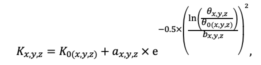
where K0 is thermal diffusivity of dry soil; θ0 is volumetric moisture at which maximum thermal diffusivity is reached; K0 + a is maximum thermal diffusivity at θ = θ0; and b is a parameter characterizing the width of the curve peak and determined by the range of moisture in which active thermal transfer of soil moisture occurs. The above parameters for organomineral horizons can be expressed through soil density and soil organic carbon content (Lukyashchenko, Arkhangelskaya, 2018):
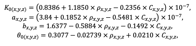
where C is carbon concentration (%). The corresponding parameters for the organogenic soil horizon were taken as constants according to the T. A. Arkhangelskaya and A. A. Gvozdkova (2019). The calculation of the thermal diffusivity of snow is described above.
Dynamics of soil organic matter pools
The Romul_Hum soil organic matter dynamics submodel is integrated into the model system (Chertov et al., 2017a, 2017b; Komarov et al., 2017a). This is a new version of the ROMUL soil model, which has been described in detail previously (Chertov et al., 2001; Modeling Dynamics …, 2007). The main difference between the Romul_Hum model and the original ROMUL model is the new procedure for calculating nitrogen dynamics. In ROMUL, as in most other models, N dynamics were strictly linked to carbon transformation pathways of soil organic matter (OM), and empirical correction factors for carbon transformation rates were used to calculate N pools. The Romul_Hum model additionally implemented procedures describing the transformation of C and N in the food webs of soil micro-, mesofauna and earthworms. By-products of soil fauna activity, in addition to exhaled C‑CO2, are organic matter of excreta, coprolites and mortmass and mineral nitrogen (mainly ammonium) of liquid excreta, which allowed more detailed calculation of soil mineral nitrogen production in Romul_Hum.
The structure of the Romul_Hum model reflects the functional activity of three communities of soil destructors. OM is represented in the model by a cascade of fractions that generally correspond to organogenic soil subhorizons (L — fresh surface litter; F — partially decomposed fermented litter; H — humified forest litter horizon) and the humus-accumulative horizon of mineral soil Ah/Ahe. The rate of mineralization in each pool was determined experimentally and depends on the chemical properties of organic matter, soil moisture and temperature (Modeling Dynamics …, 2007).
The dynamics of carbon and nitrogen pools in each cell is described by the following system of equations:
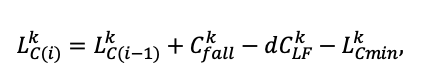
where Lkc(i) is carbon stock in cohort k of pool L at step i, is carbon entering cohort k with litter, is carbon flux from cohort k of pool L to pool F, and is C-CO2 flux from cohort k of pool L.
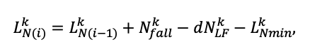
where LkN(i) is nitrogen stock in cohort k of pool L at step i, is nitrogen entering with litter, is nitrogen flux from cohort k of pool L to pool F, and is mineralized nitrogen flux from cohort k of pool L.
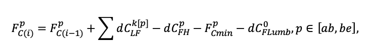
where Fpc(i) is carbon stock in cohort p (organogenic and organomineral horizons) of pool F at step i, is C‑CO2 flux from cohort p of pool F, is carbon flux consumed by earthworms from aboveground cohort F; and ab, be are hereinafter referred to as indices showing whether the pool/flux is above- or belowground.
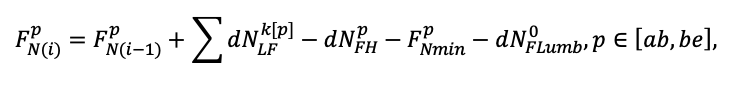
where FpN(i) is nitrogen stock in cohort p (organogenic and organomineral horizons) of pool F at step i, is mineralized nitrogen flux from cohort p of pool F, and is nitrogen flux consumed by earthworms from aboveground cohort F.
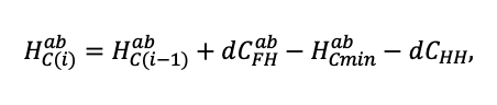
where Habc(i) is carbon stock in pool H of the organogenic horizon at step i, is C‑CO2 flux from pool H of the organogenic horizon, and dCHH is carbon flux from pool H of the organogenic horizon to the organomineral horizon.
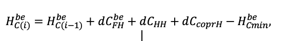
where Hbec(i) is nitrogen stock in pool H of organogenic horizon at step i, is mineralized nitrogen flux from pool H of organogenic horizon, and dNHH is nitrogen flux from pool H of organogenic horizon to organomineral horizon.
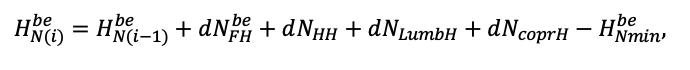
where HbeN(i) is carbon stock in pool H of the organomineral horizon at step i, is C‑CO2 flux from pool H of the organomineral horizon, and dCCoprH is carbon flux from earthworm coprolites to pool H of the organomineral horizon.
where HbeN(i) is nitrogen stock in pool H of organomineral horizon at step i, is mineralized nitrogen flux from pool H of organomineral horizon, dNcoprH is nitrogen flux from earthworm coprolites to pool H of organomineral horizon, and dNLumbH is nitrogen flux from earthworm mortmass to pool H of organomineral horizon.
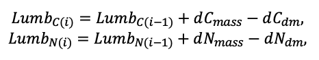
where LumbC(i) and LumbN(i) are carbon and nitrogen of earthworm biomass, dCmass and dNmass are carbon and nitrogen gains of earthworm biomass, and dCdm and dNdm are carbon and nitrogen of earthworm mortmass.
Mineralization and humification of pool L are characterized as follows:
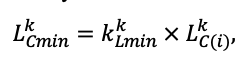
where kkLmin is mineralization coefficient of OM mineralization of cohort k of pool L.
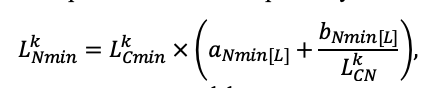
where aNmin[L] and bNmin[L] are empirical coefficients characterizing the ratio and activity of the bacterial and fungal component of the microbial community; is C:N ratio of cohort k of pool L.
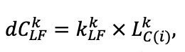
where kkLF is OM humification coefficient of cohort k of pool L.
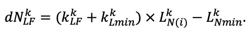
Mineralization and humification of pool F are characterized as follows:
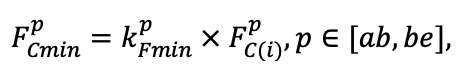
where kpFmin is OM mineralization coefficient of cohort p of pool F.
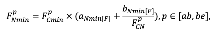
where aNmin[F] and bNmin[F] are empirical coefficients characterizing the ratio and activity of the bacterial and fungal component of the microbial community; is C:N ratio of cohort p of pool F.
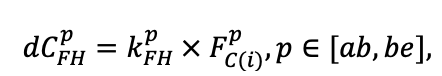
where kpFH is OM humification coefficient of cohort p of pool F.
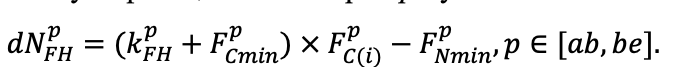
Carbon and nitrogen fluxes consumed by earthworms from pool F are calculated as
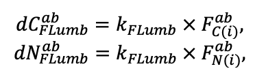
where kFLumb is the coefficient of earthworm food activity.
Mineralization and humification of pool H is characterized as follows:
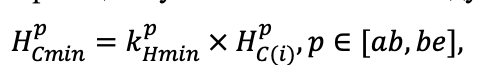
where kpNmin is OM mineralization coefficient of cohort p of pool H.
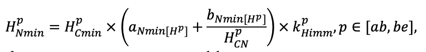
where aNmin[F] and bNmin[F] are empirical coefficients characterizing the ratio and activity of bacterial and fungal components of microbial community, is nitrogen immobilization coefficient from H pool (equal to 1.0 for organogenic horizon and 0.7 for organomineral horizon).
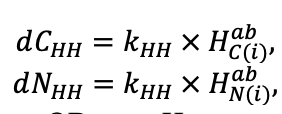
where kHH is OM humification coefficient of pool H of organogenic horizon.
Earthworm life activity is described by the following system of equations:
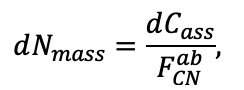
where dCass is the assimilated part of carbon consumed by earthworms, which is calculated by the equation
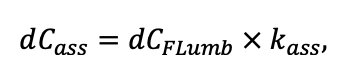
where kass is the assimilation coefficient.
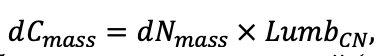
where LumbCN is the C:N ratio of earthworm biomass (taken equal to 4).
The part of carbon consumed by the worms returned to the soil with coprolites is calculated by the equation
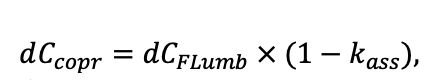
and, accordingly, the part of nitrogen consumed by worms is calculated by the equation:
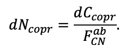
C‑CO2 mass released as a result of mineralization of earthworm coprolites is calculated as
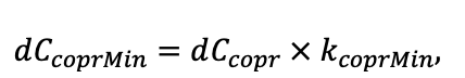
where kcoprMin is coprolites mineralization coefficient. Nitrogen in coprolite mineralization is calculated by the equation

where kNfix is the nitrogen fixation coefficient, accepted as 1.014 × 10⁻⁶ (Komarov et al., 2017a).
Carbon and nitrogen inputs from earthworm coprolites to pool H are calculated using the equations:
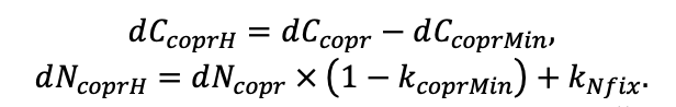
Carbon and nitrogen contents in earthworm mortmass are calculated as
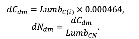
Nitrogen input from worm mortmass to the pool H of the organomineral horizon is calculated as
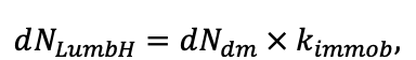
where kimmob is nitrogen immobilization coefficient.
C‑CO2 of earthworm respiration is calculated as
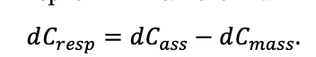
Total C‑CO2 emission due to earthworm activity is calculated as
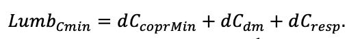
Total release of nitrogen in mineral forms resulting from earthworm activity is calculated as

The numerical values of the coefficients and corrections in the equations are borrowed from the description of the Romul_Hum model (Komarov et al., 2017a; Chertov et al. 2017a, 2017b) or compiled from other sources (Modeling Dynamics …, 2007).
Mineralization coefficient of pool L of organogenic horizons is calculated as

where Nkconc is nitrogen concentration in the litter cohort k; is (hereinafter) correction for soil temperature and moisture, and corrpH is the correction for soil pH, which is calculated as

where pH is the pH value of the soil.
Mineralization coefficient of pool L of organomineral horizons is calculated as follows
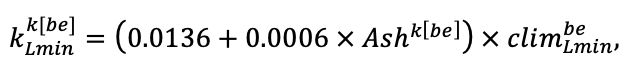
where Ashk[be] is the ash content of organic matter in the litter cohort k.
Humification coefficient of the pool L of organogenic horizons is calculated by the equation
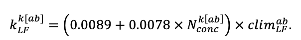
Humification coefficient of pool L of organomineral horizons is calculated as follows

Earthworm food activity coefficient is calculated by the equation
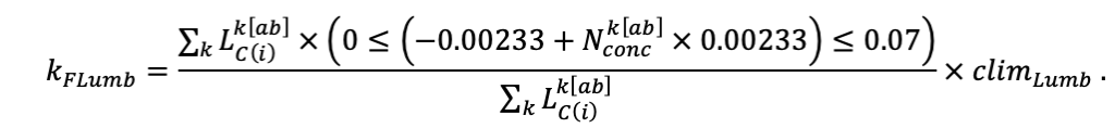
Earthworm food assimilation coefficient is calculated as
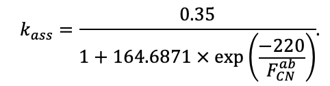
Mineralization coefficient of fresh earthworm coprolites is calculated by the equation
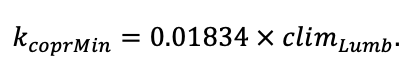
Mineralization coefficients of pools F of organogenic and organomineral horizons are calculated by equations:
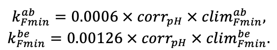
Humification coefficients of pools F of organogenic and organomineral horizons are calculated by the equation
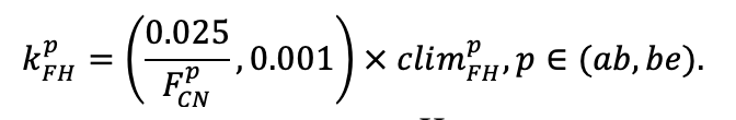
Mineralization coefficients of pools H of organogenic and organomineral horizons are calculated by equations:

where Clay is clay fraction share.
Humification coefficient of pool H of organogenic horizon is calculated as follows
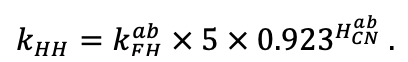
For calculation of coefficient corrections for soil moisture, the value of soil moisture standardized by field moisture capacity is used, and it is as follows:
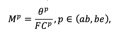 where Θp is the volumetric moisture of horizons p, and FCp is the field capacity of horizon p.
Soil moisture correction for calculation of L, F, H pools mineralization coefficient (MpLmin , MpFmin and , MpHmin respectively) and pool humification coefficient L (MpLF ) is calculated as follows:

The following equation is used to calculate the F pool humification coefficient correction:
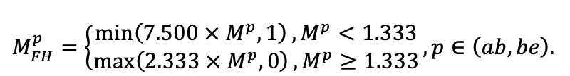
Soil moisture correction of earthworm activity coefficient is calculated as
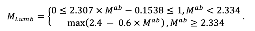
Soil temperature correction for calculation of L pool mineralization coefficient is calculated by the equation
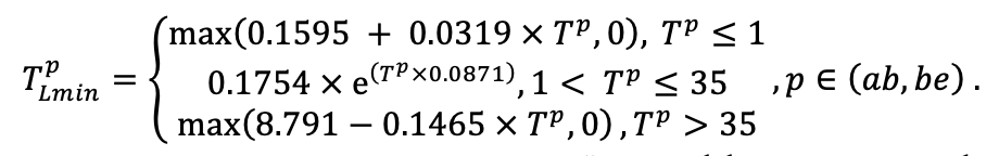
Soil temperature correction for calculation of L pool humification coefficient is calculated as

Soil temperature correction for calculation of F pool mineralization coefficient is calculated by the equation
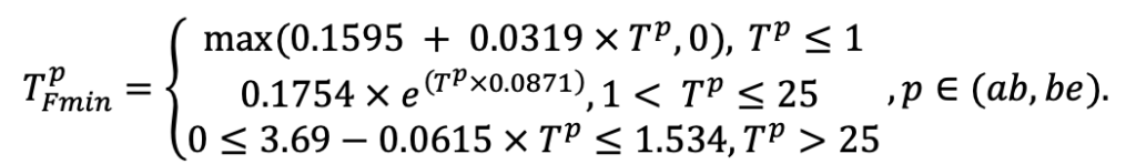 Soil temperature correction for calculation of F pool humification coefficient is calculated by the equation
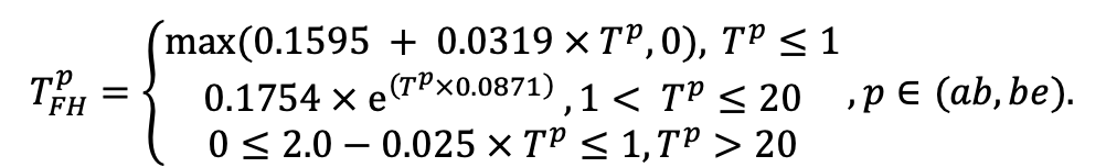 Soil temperature correction for calculation of H pool mineralization coefficient is calculated by the equation
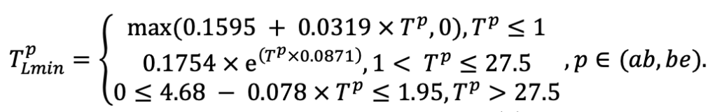 Soil temperature correction for earthworm activity coefficient is calculated as
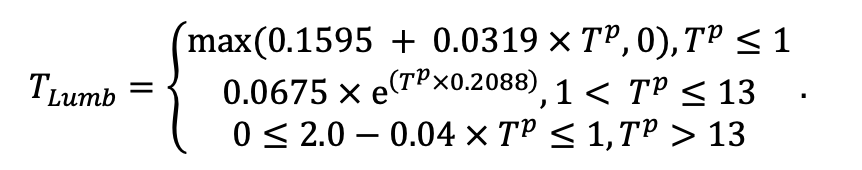 Resulting climatic corrections used in the calculation of the coefficients are calculated as the product of the temperature and soil moisture corrections.
Decomposition of coarse woody debris (CWD) in the current version of the model system is described using the same procedures as decomposition of non-timber litter fractions.
Felling simulation unit
This unit allows to simulate different types of harvesting based on specified external parameters, the main ones being harvesting intensity (removal of wood and other phytomass fractions) and methods of tree removal. The intensity of removal can be determined either as a fraction of the target value (stand basal area, m2 ha−1, or stand density, trees ha−1) before felling, or as a target value to be achieved after felling. Selection of trees for felling is based on their sorting by trunk diameter at breast height. Depending on the parameter, felling will be done either in descending order (i.e. the largest trees will be cut), in ascending order (small trees will be cut first), or trees of all diameter classes will be randomly selected for felling. In addition, it is possible to set the proportion of the largest trees that will not be cut and the threshold value of trunk diameter at breast height below which trees will not be cut even if the required removal rate is not achieved. Advanced felling algorithms involve optimizing stand thinning in such a way as to reduce competition between trees for resources. The size-to-distance ratio index is used to assess the intensity of competition and has shown good results with minimal computational complexity (Shanin et al., 2021a). The procedure parameters allow specifying the order in which trees of different species will be cut, as well as blocking the felling of trees of certain species. It is also possible to simulate leaving felling residues on the site, which are then added to the amount of plant litter and transferred to the soil organic matter dynamics submodel. Additional planting of trees in an existing stand is simulated by the same procedure as the initial placement, but taking into account the cells already occupied by trees.
Promising directions for improving the model system
The goal of any model is to provide the most accurate reproduction of basic ecosystem processes while minimizing the number of input parameters required (avoiding the need for difficult-to-define object-specific parameters in the first place). From our point of view, some improvements can be made to the model system.
First of all, a natural regeneration simulation unit is needed. In simulation experiments with the current version of the model system, for this purpose we used a procedure similar to the procedure for simulating initial tree placement using expert judgment of the density and species composition of natural regeneration. We have previously (Juutinen et al., 2018; Shanin et al., 2021b) used empirical renewal models (Pukkala et al., 2012). However, parameter estimation of these models was carried out on the basis of a limited set of experimental data, which does not guarantee their accuracy in other ecological and geographical conditions. A solution could be the development of a process model of regeneration that takes into account the seed production of trees depending on habitat conditions, seed dispersal over the simulated site (including the possibility of introducing seeds of species not present in the simulated site at the moment) and the probability of successful establishment and survival of the undergrowth depending on local conditions (canopy illumination, moisture, presence of grass-shrub layer plants). This submodel should also include the ability to simulate vegetative propagation using data on root system distribution and rootstock formation rates.
Both the regeneration submodel and the initial tree placement simulation procedure can be improved by detailed more sophisticated procedures that account for spatial clustering of trees of the same or different species (Pommerening, Grabarnik, 2019). To expand the range of possible simulation scenarios, it is necessary to include in the model system procedures that simulate different types of disturbances such as fires, windthrow, phytopathogens and pollution. The existing simulated felling procedure can be improved by implementing optimization procedures (Tahvonen, Rämö, 2016) that automatically select felling parameters to maximize the target, which can be maximum income, carbon storage, etc. In addition, the optimization algorithm for selecting trees for felling can use the outputs of competition submodels (i.e., the amount of resources obtained by each tree) instead of the simplified competition index to calculate the optimal thinning of the stand. In the competition submodel, it should be possible to simulate competition for elements of soil nutrition and water (other than nitrogen).
The current version of the model system uses a static approach to micro-relief generation, performed only during the initialization phase. A transition to a dynamic submodel is needed, with two main areas of development being the simulation of microrelief changes over time and the influence of microrelief on tree regeneration and grass-shrub layer vegetation. The current version of the litter distribution submodel does not take into account the heterogeneity of biomass distribution within crowns, as well as the influence of the spatial structure of the tree canopy and microrelief on litter distribution, hence the need to refine these procedures.
Experience gained in modeling stand dynamics on drained peatlands (Shanin et al., 2021b) has shown the importance of considering the water table and its influence on tree stand productivity, and tree regeneration success. It is also necessary to modify soil organic matter dynamics submodel to simulate decomposition of a portion of in-soil litter under anaerobic conditions.
Soil organic matter submodel considers the dynamics of labile and stable carbon pools, while carbon in “superstable” states, such as deep soil organic matter and pyrogenic carbon (Lehmann, Kleber, 2015), is not considered in the submodel, which may lead to more distinct fluctuations in soil organic matter stocks with changing vegetation formations than actually observed (Luyssaert et al., 2008). As a consequence, a necessary addition in the development of the submodel, especially important for long-term forecasting, is the inclusion of an corresponding pool in the soil organic matter submodel. Another promising direction of submodel development is the inclusion of cycles of other elements (primarily phosphorus and calcium) into the model system, using already existing developments (Khoraskina et al., 2010; Komarov et al., 2012), as well as modeling the dynamics of the corresponding elements in the stand and grass-shrub layer. To better account for the interrelationships between different components of forest ecosystems, the inclusion of units for simulating rhizosphere priming effect (Priputina et al., 2021; Chertov et al., 2022) and mycorrhiza in the model system is also suggested. It is also obvious that a separate submodel is needed to take into account the relationship between CWD size and decomposition rate, as well as the peculiarities of specific CWD fractions (standing dead trees, fallen logs) (Didion et al., 2014; Shorohova, Kapitsa, 2014).
Currently, species-specific parameters were estimated only for the following 12 main species: Pinus sylvestris, Picea abies, Larix sibirica, Abies sibirica, Betula pendula / Betula pubescens (parameters for both species were assumed to be identical), Populus tremula, Quercus robur, Tilia cordata, Fagus sylvatica, Acer platanoides, Ulmus glabra, Fraxinus excelsior. Accordingly, another area of work is to continue parameterization of the model system (including both estimation of parameters for other tree species and refinement of existing parameter values) to more accurately model the dynamics of mixed stands.
SIMULATION EXPERIMENTS
Simulation scenarios
To test the correctness of the model system, a set of scenarios was constructed to simulate stands with different species composition, different spatial structure and at different stages of development. The simulation experiments were conducted on a 100 × 100 m virtual site divided into 0.5 × 0.5 m cells. Simulation scenario parameters are summarized in Table 6. Soil-climatic conditions were assumed to correspond to C3 forest site type (Zheldak, Atrokhin, 2002) for the subzone of coniferous-broadleaved forests.
Table 6. Initial parameters of simulation scenarios
| Code | Tree stand formula | Stand density, trees ha−1 | Mean height, m | Mean trunk diameter at breast height, cm | Age, years | Type of tree placement in space |
| 1. P_Yr | 10P | 4400 | 4.5 ± 0.2 | 6.0 ± 0.3 | 10 | Pseudorandom |
| 2. B_Yr | 10B | 4400 | 4.5 ± 0.2 | 6.0 ± 0.3 | 10 | Pseudorandom |
| 3. P5B5_Yr | 5P5B | 4400 | 4.5 ± 0.2 | 6.0 ± 0.3 | 10 | Pseudorandom |
| 4. P7B3_Yr | 7P3B | 4400 | 4.5 ± 0.2 | 6.0 ± 0.3 | 10 | Pseudorandom |
| 5. P3B7_Yr | 7B3P | 4400 | 4.5 ± 0.2 | 6.0 ± 0.3 | 10 | Pseudorandom |
| 6. P_Yc | 10P | 4400 | 4.5 ± 0.2 | 6.0 ± 0.3 | 10 | Clustered |
| 7. B_Yc | 10B | 4400 | 4.5 ± 0.2 | 6.0 ± 0.3 | 10 | Clustered |
| 8. PB_Yc | 5P5P | 4400 | 4.5 ± 0.2 | 6.0 ± 0.3 | 10 | Clustered |
| 9. P_Yg | 10B | 4400 | 4.5 ± 0.2 | 6.0 ± 0.3 | 10 | Regular |
| 10. B_Yg | 10B | 4400 | 4.5 ± 0.2 | 6.0 ± 0.3 | 10 | Regular |
| 11. PB_Yg | 5P5B | 4400 | 4.5 ± 0.2 | 6.0 ± 0.3 | 10 | Regular |
| 12. P_Mr | 10P | 400 | 27.7 ± 1.2 | 33.4 ± 2.3 | 100 | Pseudorandom with threshold distance |
| 13. S_Mr | 10S | 400 | 27.7 ± 1.2 | 33.4 ± 2.3 | 100 | Pseudorandom with threshold distance |
| 14. B_Mr | 10B | 400 | 27.7 ± 1.2 | 33.4 ± 2.3 | 100 | Pseudorandom with threshold distance |
| 15. PS_Mr | 5P5S | 400 | 27.7 ± 1.2 | 33.4 ± 2.3 | 100 | Pseudorandom with threshold distance |
| 16. PB_Mr | 5S5B | 400 | 27.7 ± 1.2 | 33.4 ± 2.3 | 100 | Pseudorandom with threshold distance |
| 17. L_Mr | 2O2L2M2E2A | 400 | 27.7 ± 1.2 | 33.4 ± 2.3 | 100 | Pseudorandom with threshold distance |
| 18. PS_Tr | I: 10P | 400 | 27.7 ± 1.2 | 33.4 ± 2.3 | 100 | Pseudorandom with threshold distance |
| II: 10S | 1000 | 5.0 ± 0.5 | 10.0 ± 1.0 | 30 | Pseudorandom | |
| 19. BL_Tr | I: 10B | 400 | 27.7 ± 1.2 | 33.4 ± 2.3 | 80 | Pseudorandom with threshold distance |
| II: 2O2L2M2E2A | 1000 | 5.0 ± 0.5 | 10.0 ± 1.0 | 30 | Pseudorandom | |
| 20. PSL_Tr | I: 4P4S2B | 300 | 27.8 ± 2.9 | 40.7 ± 9.5 | 100 | Pseudorandom with threshold distance |
| II: 5S4L1O | 700 | 12.3 ± 6.6 | 13.8 ± 2.8 | 30 | Clustered | |
| 21. L_Tr | I: 2O2L2M2E2B | 300 | 28.0 ± 2.9 | 41.0 ± 9.6 | 50–150* | Pseudorandom with threshold distance |
| II: 4E3L3M | 400 | 10.4 ± 1.3 | 15.1 ± 2.1 | 30 | Pseudorandom | |
| 22. S_Ur | 10S | 700 | 2.0–33.0* | 2.4–55.8* | 10–200* | Pseudorandom |
Note: “I”, “II” are the indicators of separate stand layers. Mean height and mean trunk diameter at breast height are shown for mean ± standard deviation. Type of tree placement in space is the following: pseudorandom, pseudorandom with threshold distance (priority of stand density); clustered; by regular scheme (4.5 m between rows, 0.5 m between seedlings in a row). * — the value range is specified. P — Pinus sylvestris, S — Picea abies, B — Betula spp., O — Quercus robur, L — Tilia cordata, M — Acer platanoides, E — Ulmus glabra, A — Fraxinus excelsior.
Results of the simulation experiments were analyzed by a set of control variables including the following: (a) PAR interception at the individual tree level (MJ per 1 kg of absolutely dry foliage biomass); (b) distribution of under PAR under canopy at the individual cell layer (as a fraction of above-canopy PAR); (c) N uptake in plant-available forms at the individual tree layer (in g per 1 kg of absolutely dry fine root biomass); (d) overlap of tree root systems at the level of individual cells; (e) net primary production of stands during the growing season, kg ha−1; (f) heterogeneity of spatial distribution of soil hydrothermal characteristics. When analyzing the productivity of stands of the same structure but with different species composition, the effect of “overyielding” (Loreau, 1998) was also analyzed, based on the calculation of the ratio of predicted productivity of a mixed stand to its theoretical expected productivity. The latter is defined as a weighted average of the predicted productivity values of the corresponding single-species stands, where the weight measure is the proportion of species in the analyzed mixed stand (Pretzsch et al., 2013). Thus, the values of additional productivity exceeding 1 show the influence of the “niche segregation” effect on the productivity growth of mixed stands compared to single-species stands. When analyzing the spatial heterogeneity of hydrothermal characteristics of soils, the data of meteorological station Kolomna for 1976 were used. Two days in spring and summer periods were selected for which the influence of spatial heterogeneity on the hydrothermal regime is most evident. On the 100th day of the year (09.04.1976) the snow cover on the open ground and under deciduous stands has already melted, and under coniferous stands it has not yet melted. The vegetation of deciduous trees and living ground cover plants has not yet begun. Mean daily air temperature is +4.5 ºC. On the 210th day (27.06.1976) mean daily air temperature is 20.0 ºC, and daily precipitation is 10 mm. The preceding week was warm (mean daily temperatures were 17.1–20.6 ºC) and practically without precipitation. However, 32 mm of rainfall had fallen earlier during the two days, but over a week of warm and dry weather this amount of water must have been largely used up for evapotranspiration.
The initial meteorological information required for the soil hydrothermal regime submodel (air temperature, precipitation, and air humidity characteristics (saturation deficit and relative humidity of daily resolution) was obtained from data sets prepared at the All-Russian Research Institute of Hydrometeorological Information — World Data Center (RIHHMI — WDC) of Roshydromet and available at http://meteo.ru/data. For characterizing climatic conditions, data of the meteorological station Kolomna were used. The 30-year period of 1981–2010 was chosen as the baseline period to assess the statistical characteristics of the present-day climate. Stationary climate scenarios were then generated by randomly sampling full years of data (in order to preserve both intra-annual parameter autocorrelation and correlation between parameters) until reaching 70-year durations (in daily time steps). Obtained scenarios were checked for the absence of tendencies both by visual inspection of indicator diagrams and by approximation of indicators by a linear function (the absence of significant differences in the slope coefficient of the linear function from 0 was checked). Initial stocks of OM and nitrogen in organic and organomineral soil horizons in the simulation experiments were the same for all cells of the simulated forest site. Stock estimates were made based on field soil survey data by the authors in Prioksko-Terrasny Nature Reserve. Spatial differentiation of soil reserves of OM and nitrogen in the simulation experiment occurred due to the input of different amounts of species-specific fractions of plant litter into the cells of the model grid and the dependence of the intensity of its transformation (mineralization) on the hydrothermal conditions of the corresponding soil horizons. Grass-shrub layer was represented by the following 5 species: Calamagrostis arundinacea, Convallaria majalis, Pteridium aquilinum, Vaccinium myrtillus and Vaccinium vitis–idaea. Three scenarios of stand development were modeled. The first scenario is a polydominant stand of Pinus sylvestris, Picea abies, Betula spp. and Populus tremula with a pseudorandom arrangement of trees. Initial C and N reserves in the organic horizon are as follows: 2.625 kg m−2 (C), 0.054 kg m−2 (N), and in the organomineral horizon they are 3.14 and 0.19 kg m−2, respectively. The second scenario is a pine-birch stand with trees arranged in several dense clusters. Initial C and N stocks in soil are similar to the previous scenario. The third scenario is Pinus sylvestris species with trees arranged in a regular square grid with 2 × 2 m spacing. It was assumed that the organogenic horizon of soils was strongly disturbed as a result of the formation of planting furrows, and the initial C and N reserves correspond to those in the organomineral part of the profile and as follows: C is 1.393 kg m−2, and N comprises 0.103 kg m−2.
In addition to undisturbed forest ecosystem scenarios, the effects of external forcing factors were simulated. They included a selective felling with removal of 30% of the largest trees (based on the sum of cross-sectional areas), climate change (under RCP 4.5, RCP 6.0 and RCP 8.5 scenarios from the IPCC 5th Assessment Report (IPCC, 2013)), and a 50% increase in the input of N compounds from precipitation compared to the baseline (Jia et al., 2016).
Results and discussion
To compactly represent spatially distributed indicators (at the level of individual trees or cells of the simulation grid) at a single point in time, a variogram is used, which depicts the distributions of analyzed indicators for several simulation scenarios using probability density curves. The width of each curve corresponds to the approximate frequency of data points with the corresponding index value on the ordinate axis. Horizontal lines on the variogram are consistent with the median values of the corresponding indicators. To represent the dynamics of the spatial distribution of indicators at the cell level of the simulation grid, a diagram is used, which is a vertical sequence of probability density distributions of the analyzed indicator for different simulation steps, aligned on a horizontal scale. All presented results should be considered as preliminary, since at this stage the main purpose of simulation experiments was to test the functional capabilities of the model system to reproduce the functional relationships between different components of forest ecosystems, taking into account the influence of spatial heterogeneity at different levels, and not to demonstrate the application of the model system to solve specific practical or research problems. In this regard, temporal dynamics is demonstrated only for those indicators on which the influence of spatial heterogeneity is cumulative.
Competition for resources and productivity of forest stands
Results analysis of the simulation experiments revealed a number of aspects in the functioning of the modeled forest ecosystems. It is shown that the intensity of root competition in a stand depends more on its species composition and spatial structure than on its age, although there is a slight increase in the intensity of competition for soil nutrition elements in mature stands compared to young stands (Fig. 15). At the same time, as the age of the stand increases, homogeneity in the spatial distribution of competition density increases as well. This is explained by the fact that the multiplicity of root system overlap significantly exceeds the multiplicity of crown projection overlap, which was shown earlier (Sannikov, Sannikova, 2014). Such density of root system overlap is primarily due to the high range of root horizontal spread relative to the size of the crown and, as a consequence, to a much higher area of the tree root system compared to the area of its crown projection.
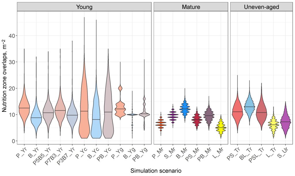
Figure 15. Distribution of root competition intensity (number of nutrition zone overlaps per 1 m2 of simulation grid) in stands of different composition and spatial structure. Codes and characteristics of the scenarios are summarized in Table 6. Horizontal lines indicate median values
Differences in initial tree location also influence nature of root competition. With a pseudorandom initial arrangement of trees, the distribution of nutrition zone overlap is close to normal. When trees are clustered, this distribution is bimodal, with one peak (in the region of high intensity of competition) corresponding to groups of trees with a dense arrangement, and a second peak in the region of gaps between such clusters, where the intensity of competition is low. When trees are arranged according to a regular grid, there are several peaks associated with a higher density of overlapping nutrition zones within the rows and a lower density in the inter-rows. In mature stands with one layer, the density of nutrition zone overlap is lower than in stands with a more complex tree stand structure (Fig. 15).
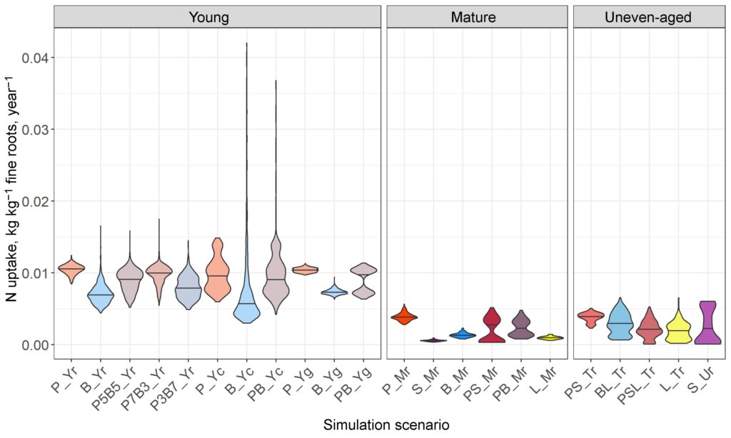
Figure 16. Total annual nitrogen consumption at the level of individual trees, kg per 1 kg of fine root biomass, in stands of different composition and spatial structure
According to model estimates, N uptake by trees decreases with increasing age as follows: from about 0.010 kg N per 1 kg of fine root biomass per year in young stands to 0.002–0.005 in mature stands. Uneven-aged and mixed stands demonstrate more efficient resource use (due to more uniform distribution of underground organs biomass) compared to single-aged mono-species stands. The spatial structure does not significantly affect the median value of this indicator, but influences the nature of its distribution (Fig. 16). Lower values of N consumption in uneven-aged stands, in addition to the model system’s inherent decrease in N consumption efficiency as trees age, can be explained by stronger competitive pressure from large trees. N uptake in spruce forests is also additionally influenced by a higher root saturation in the soil compared to other stands, which can be explained by a higher proportion of fine root biomass (of total tree mass) in Picea abies compared to trees of other species (Helmisaari et al., 2002). Moreover, in most of the mixed stands, the value of N consumption was higher than expected, which can be calculated as an arithmetic mean between the consumption rates in pure stands formed by the species included in a given mixed stand. This, in our opinion, confirms the effective realization of the mechanisms of simulating “niche segregation” embedded in the model system, which consist, in particular, in the fact that aboveground and underground organs of trees of different species differ in the nature of vertical distribution, thereby reducing the intensity of competition and increasing the efficiency of resource use (Cavard et al., 2011; Pretzsch et al., 2015).
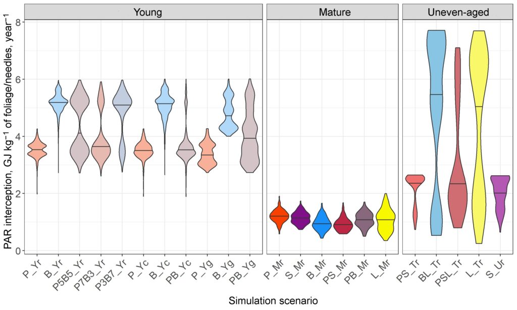
Figure 17. PAR interception at the level of individual trees (GJ per 1 kg of foliage/needles, sum for the growing season) in stands of different composition and spatial structure
In general, the simulation experiments showed higher PAR interception by deciduous trees (per 1 kg of foliage biomass) compared to coniferous trees. The values of this index are higher for the young-growth stage, which we attribute to the more sparse placement of trees and less shading of leaves (needles) in the lower canopy layers compared to mature and uneven-aged stands. Tree placement according to a regular grid influenced a different distribution pattern and median value of PAR interception in young trees, compared to pseudorandom and clustered placement. The main influence here is the mutual shading of trees within the row, which cannot be fully compensated for by the expansion of crowns in the direction of the row spacing (Fig. 17). The median value of PAR interception is higher in uneven-aged stands compared to mature stands.
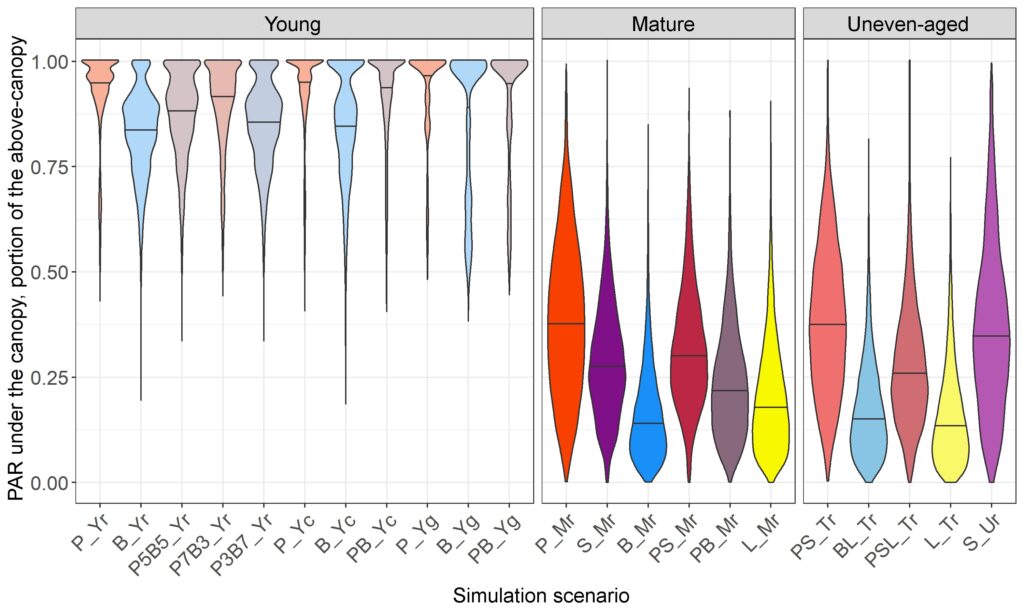
Figure 18. Distribution of PAR reaching the soil surface (fraction of the aboveground PAR) at the level of individual cells of the simulation grid in stands of different composition and spatial structure
Thus, in clustered placement, resource development both at the level of individual trees and at the level of the stand as a whole is less efficient. Since on the one hand, competition in dense groups is very high, which limits the amount of resources at the level of an individual tree, and on the other hand, the possibility of germination into the “gaps” of root systems and especially tree crowns is limited. The placement of trees according to a regular grid in some cases was even more efficient than pseudorandom placement in terms of resource utilization. However, the peculiarities of these stands, related to their lower stability, should be taken into account. In the development of stands with such a structure, the intensity of competition has similar indicators for all trees, which can lead at a certain stage to their mutual oppression and subsequent intensive self-thinning (Priputina et al., 2016). The death of some trees in stands with such a structure creates large gaps in the canopy, which cannot be compensated by lateral expansion of the crowns of the nearest trees. At the same time, in stands with a pseudorandom arrangement of trees (even mono-species and single-age stands), a number of trees have an advantage due to lower competitive pressure on them from neighboring trees, which at the stand level may contribute to more efficient consumption of resources, as well as increase the resistance of such stands to self-thinning.
Analysis of PAR distribution under the canopy showed, as expected, that there are no heavily shaded areas in young trees. In coniferous stands, the proportion of well-lit areas is higher, which is explained by more compact crowns, which (with the same stand density and tree size assumed in all simulation scenarios) give more “gaps” in the canopy. In mature coniferous stands the distribution of PAR under the canopy is more uniform compared to mature stands of deciduous species (Fig. 18). In mature deciduous stands, the proportion of strongly shaded cells is higher.
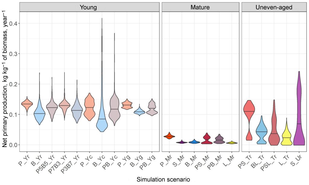
Figure 19. Productivity at the individual tree level (kg of net primary production per year per 1 kg of total tree biomass) in stands of different composition and spatial structure
The value of net primary production (in kg per 1 kg of total tree biomass) is expectedly higher in young trees. Peak productivity values in young stands with clustered placement correspond to individual trees growing in sparse sections of stands, which, as a consequence, are practically not limited by available PAR and less limited by the amount of available nitrogen. Additionally, high productivity values are observed in stands with complex structure, especially in absolutely uneven-aged spruce forest (Fig. 19). The values of additional productivity for mixed young trees are as follows: 1.028 for 7P3B, 1.036 for 5P5B, and 1.030 for 3P7B.
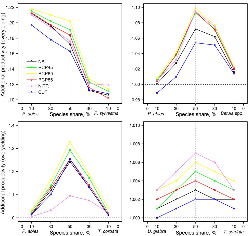
Figure 20. Projected values of additional productivity in mixed stands of different composition under no-felling scenario (NAT), climate change (RCP45, RCP60 and RCP85), increased input of nitrogen compounds from precipitation (NITR) and selective felling (CUT)
Practically in all modeled variants of mixed stands the value of additional productivity was higher than 1 (Fig. 20). The values of additional productivity in most of the impact scenarios were higher than in the undisturbed scenario, showing the higher resilience of mixed stands. The additional productivity index is also higher in stands formed by species with different ecological and cenotic strategies.
Hydrothermal conditions and soil organic matter dynamics heterogeneity
Results analysis of simulation experiments to assess the spatial variation of soil hydrothermal characteristics showed that on the 100th day of the year, soil moisture in all deciduous stands remains spatially homogeneous. In this case, in the forest floor, where the average value of soil moisture is 0.17 m3 m−3 (Fig. 21), moisture decreased in comparison with the value of 0.30 m3 m−3 set at the beginning of the simulation experiment, and in the underlying organomineral horizon increased up to 0.24 m3 m−3 (Fig. 22) in comparison with the initial of 0.20 m3 m−3.
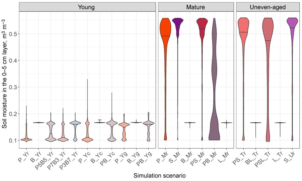
Figure 21. Moisture distribution in the 0–5 cm layer on the 100th day of the year under stands of different composition and spatial structure
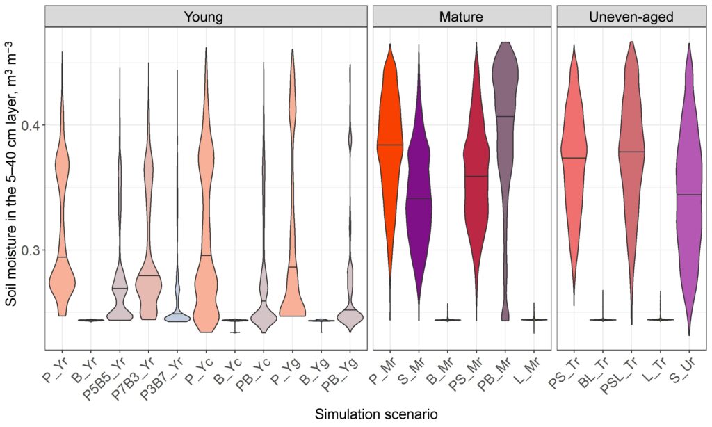
Figure 22. Soil moisture distribution in the 5–40 cm layer on the 100th day of the year under stands of different composition and spatial structure
In mixed young stands with Pinus sylvestris and Betula spp. the distribution of forest floor moisture content is bimodal, with modes, one of which is similar to the value under the deciduous stands considered above (0.17 m3 m−3), and the other corresponds to the lowest moisture content (0.10 m3 m−3). Moisture content of the organomineral horizon in this variant of stands varies in the range from values close to the lowest moisture content corresponding to this horizon (0.25 m3 m−3) to values of 0.45 m3 m−3, which is close to the full moisture content (0.49 m3 m−3); at the same time, low values spatially prevail. Apparently, rare cells with high values of moisture of the organomineral horizon correspond to areas of stronger shading, where snow melted later and not all excess moisture had time to penetrate into the underlying horizons. This can be confirmed by the picture in mature and uneven-aged coniferous stands, where, obviously, snow cover melting, due to more significant shading, has not yet ended. Accordingly, moisture distribution in the forest floor is asymmetric with a mode in the area of high values, whereas in the organomineral horizon it is closer to symmetric, i.e. on a part of the simulation site moisture has already had time to increase significantly, and on a part it has not yet, but intermediate values prevail. Spatial heterogeneity of snowmelt rates creates preconditions for the formation of loci of ephemeroid plants actively participating in the biological cycle of elements.
Forest floor temperature on day 100 was around +3.8 °C under all deciduous stands (0.7 °C below air temperature). In soil at a depth of 20 cm it was around +2.3 °C, with relatively uniform distribution in space due to more rapid snow cover melt in conditions of weak shading. Under young stands with Pinus sylvestris, the temperature values are on average almost the same with slightly greater dispersion and some minor outliers towards lower temperatures, obviously in places of later snowfall. In mature and uneven-aged stands with coniferous species, the temperature range is much wider (+0.3 … +3.9 °C in the forest floor and +0.3 … +2.4 °C at a depth of 20 cm), and the distribution is bimodal with modes close to the range edges and low repeatability of intermediate values (Figs. 23, 24). Such spatial heterogeneity is obviously caused by the non-simultaneous snow cover descent, which has not yet been completed in more shaded areas.
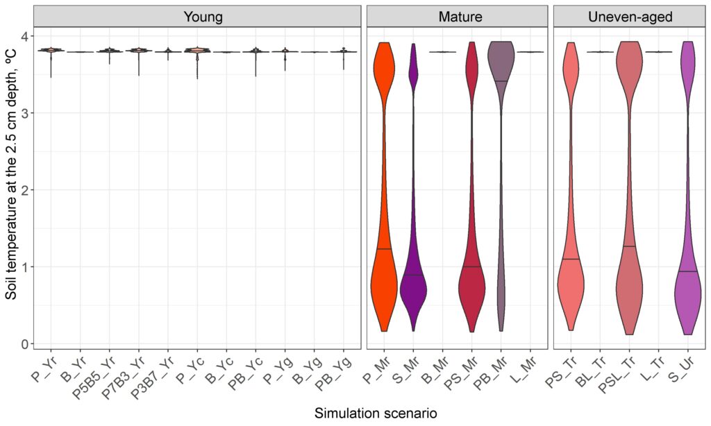
Figure 23. Temperature distribution at a depth of 2.5 cm on the 100th day of the year under stands of different composition and spatial structure
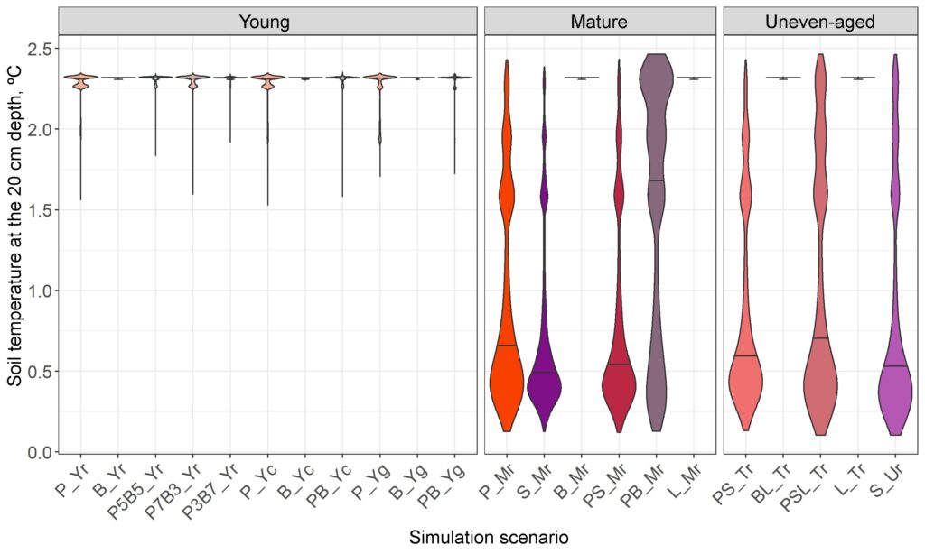
Figure 24. Soil temperature distribution at 20 cm depth on the 100th day of the year under stands of different composition and spatial structure
At day 210 under young trees, the distribution of forest floor moisture content was distinctly bimodal with maximum repeatability of values of 0.31 and 0.20–0.23 m3 m−3. In mature and uneven-aged stands, forest floor moisture values (Fig. 25) are mainly concentrated in the range of 0.14–0.24 m3 m−3, very rarely reaching maximum values close to those in young stands. In the organomineral horizon (Fig. 26) of young stands there is an asymmetric distribution with increased frequency of relatively high values (about 0.30–0.33 m3 m−3 with maximum values up to 0.35 m3 m−3 and relatively rare deviations towards lower values (0.18–0.30 m3 m−3). Under mature and uneven-aged stands the distribution of moisture values of the organomineral horizon is more diverse. Spruce forests are spatially dominated by higher moisture values with a relatively narrow range of values, while birch and pine forests have lower values with a wider range. In broad-leaved stands, the widest possible range is observed with higher values predominating.
We suppose that 10 mm of precipitation (after a week without precipitation and at increased temperature relative to the norm) noticeably manifested themselves only in young stands, whereas they had a relatively weak effect on the moisture content of forest floor and, moreover, of the organomineral soil horizon in mature and uneven-aged stands due to increased transpiration.
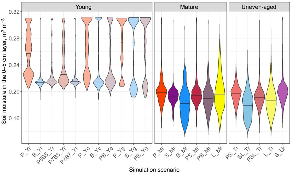
Figure 25. Moisture distribution in the 0–5 cm layer on the 210th day of the year under stands of different composition and spatial structure
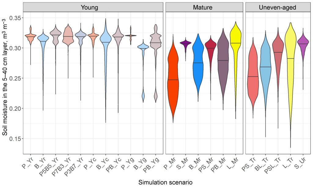
Figure 26. Moisture distribution in the 5–40 cm layer on the 210th day of the year under stands of different composition and spatial structure
According to calculations, the forest floor temperature at day 210 (Fig. 27) is 2.0–2.5 ºC and that of organomineral horizon is 7.0–7.5 ºC lower than the air temperature (Fig. 28). Spatial heterogeneity of the temperature field in young stands is less evident than under mature and uneven-aged stands.
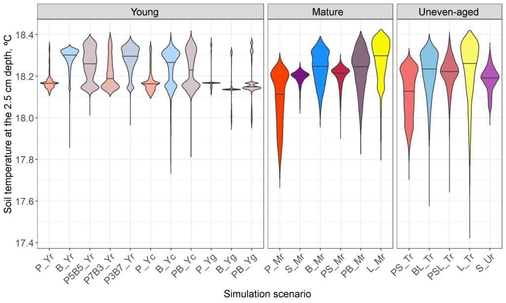
Figure 27. Soil temperature distribution at 2.5 cm depth on the 210th day of the year under stands of different composition and spatial structure
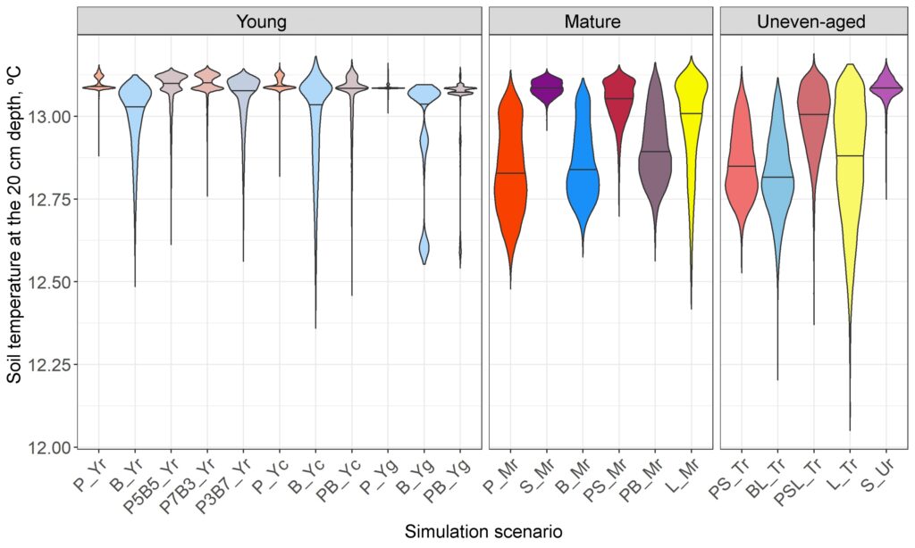
Figure 28. Soil temperature distribution at 20 cm depth on the 210th day of the year under stands of different composition and spatial structure
Results of simulation experiments to assess spatial variation of organic matter (C) and nitrogen (N) reserves in the soil cover of forest phytocenoses were analyzed based on comparison of data from three scenarios of stand development from young stands (5–10 years) to mature stands (70 years). In each of them two variants of plant litter inputs were considered and were as follows: (1) spatially localized according to stand structure species-specific litter of the tree layer only, and (2) stand litter together with that of grass-shrub layer.
In the scenario with polydominant stand of Pinus sylvestris, Picea abies, Betula spp. and Populus tremula with pseudorandom arrangement of trees, the soil and vegetation conditions of the simulated site are close to the conditions of the permanent sample plot in the Prioksko-Terrasny Reserve, where field studies were conducted. Calculation results visualization shows similar character of C and N reserves distribution in soil horizons with field data. In the predictive calculations, starting from the first modeling steps, the spatial heterogeneity of C and N pool distribution between subcrown and inter-crown areas is reproduced due to the difference in the amount of received surface litter. In simulation estimates, additional consideration of grass-shrub layer litter creates greater spatial heterogeneity of soil parameters in young and middle-aged stands with less closed crown canopy, which was reflected in the diagrams of probability distribution of carbon and nitrogen stock values (Fig. 29). By the stand age of 70 years, the distribution of OM and N stocks in forest floor is determined mainly by the nature of tree layer litter, while the influence of grass-shrub layer plants is minimal, as evidenced by similar stock distribution diagrams for the scenarios under consideration. For organomineral horizons, model calculations in both variants of litter income show greater heterogeneity in the spatial distribution of C and N reserves compared to forest floor, which is consistent with field data (Priputina et al., 2020).
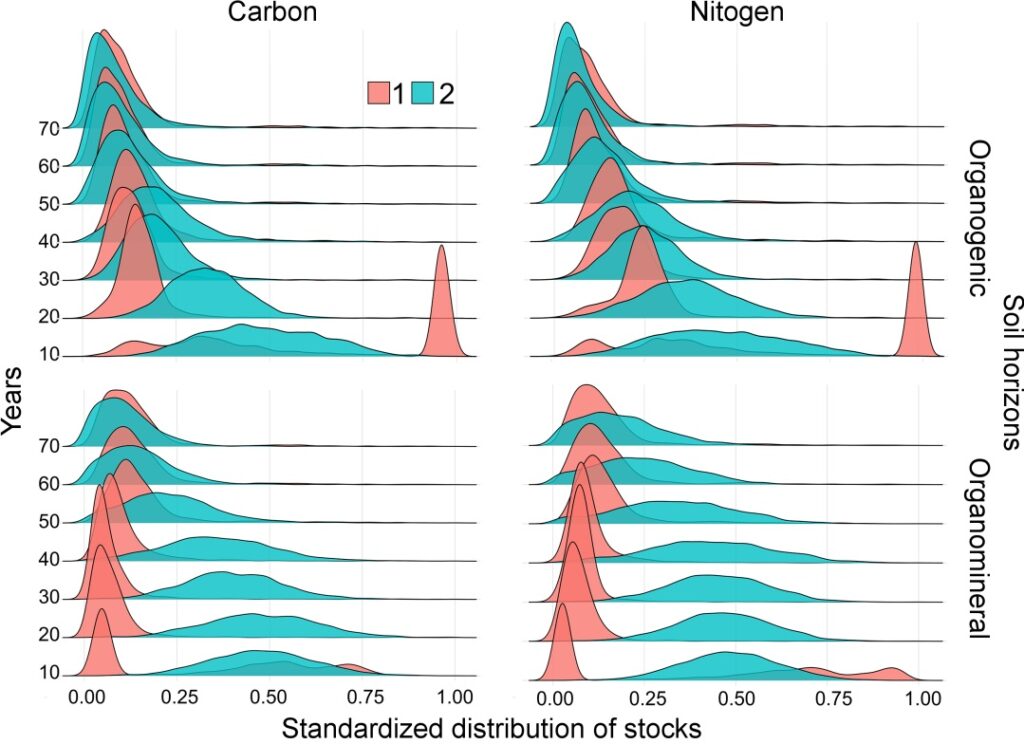
Figure 29. Standardized distribution of organic matter stocks in terms of carbon (C) and nitrogen (N) in organogenic (forest floor) and organomineral soil horizons in the scenario of polydominant stand with pseudorandom tree arrangement. 1 — only stand litter was taken into account in model calculations, 2 — including stand litter and grass-shrub layer litter. The x-axis shows standardized distribution of reserves in gradation from minimum to maximum at the site per corresponding time step
The contribution of grass-shrub layer plants to the maintenance of soil organic matter reserves is more clearly demonstrated by the data on the dynamics of averaged C and N reserves calculated as an average for the whole simulated site (Fig. 30). As it can be seen in the diagrams above, the model system shows increased C and N reserves in organic horizons (forest floor) when taking into account the grass-shrub plants litter, compared to the variant of litter input only from the tree stand. This is explained, in particular, by the fact that the submodel of soil organic matter dynamics takes into account a part of the root litter of shrubs and grasses into the forest floor. In organomineral horizons, the contribution of ground cover plants to the dynamics of organic matter reserves is less evident.
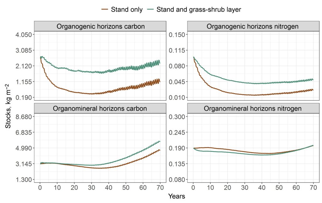
Figure 30. Dynamics of carbon and nitrogen stocks distribution in forest floor (organogenic horizons) and organomineral part of the profile in the scenario of a polydominant stand with pseudorandom tree arrangement: mean values of indicators for the corresponding soil horizons
In the scenario with clustered placement of tree species with similar ecological and cenotic strategies (Pinus sylvestris and Betula spp.), the significant role of competition for resources between closely growing trees as a factor of decreased leaf/needle production can be traced, which is reflected in reduced C and N stocks for plots within clusters formed by trees of the same species. In contrast to the polydominant stand with pseudorandom arrangement, the cluster structure of trees of different species with different N content forms a more contrasting distribution in the biogeocoenosis space of soil C and N reserves, especially at the young-growth stage, as evidenced by the presence of 2–3 peaks of standardized distribution in the scenario without taking into account the grass-shrub litter (Fig. 31). When the contribution of ground cover plants to the total plant litter pool is taken into account, the contrast in the distribution of indicators in space is slightly reduced. At the same time, as in the polydominant stand scenario, there are noticeable differences in the nature of distribution of soil C and N reserves for organogenic and organomineral horizons. The dynamics of the average C and N stocks for the simulated site are generally similar to the previous scenario (Fig. 32), but for C stocks in forest floor at the deciduous stand stage the differences between the litter variants are less distinct. This can be explained both by differences in the quality of pine-birch and polydominant stands’ litter quality and by a noticeable decrease in the contribution of grass-shrub litter to total litter due to shading under the canopy of deciduous stands.
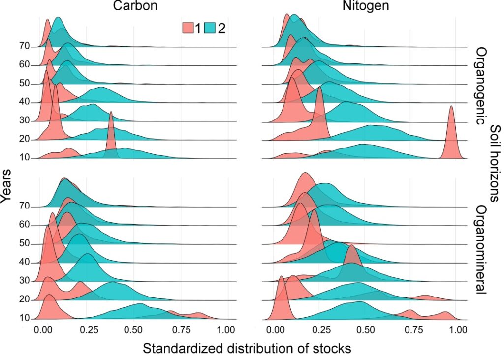
Figure 31. Standardized distribution of C and N stocks in organogenic (forest floor) and organomineral soil horizons in a scenario of a pine-birch stand with clustered tree placement. Symbols are the same as in Fig. 29
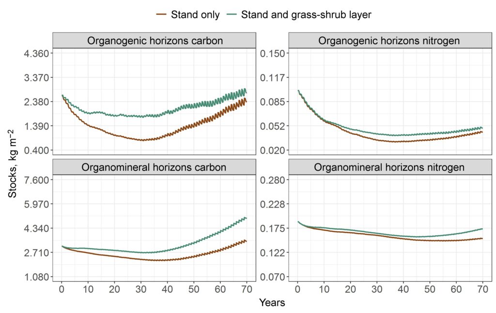
Figure 32. Dynamics of C and N stocks distribution in forest floor (organogenic horizons) and organomineral part of soil profile in the scenario of pine-birch stand with clustered placement of trees: mean values of indicators for corresponding horizons
In the scenario of Pinus sylvestris cultivation with trees placed according to a regular grid, the results of predictive assessments reflect the important role of ground cover plants in maintaining soil fertility at the initial stages of forest growth, when the mass of annual litter formed by the stand is small and its spatial distribution on the surface and in the root-inhabitable layer of soils is highly localized (Fig. 33). Noticeable differences between the distribution of indicators in organogenic and organomineral horizons are explained by the fact that in the scenario with Pinus sylvestris cultures were formed on soil with absent forest floor. The diagrams reflect the peculiarities of C and N stock accumulation and distribution during its formation, and the presence of a two-top stock distribution at the age of mature stands shown by the model system in the case of taking into account only a tree stand litter corresponds to the differences between sub-crown and inter-crown areas.
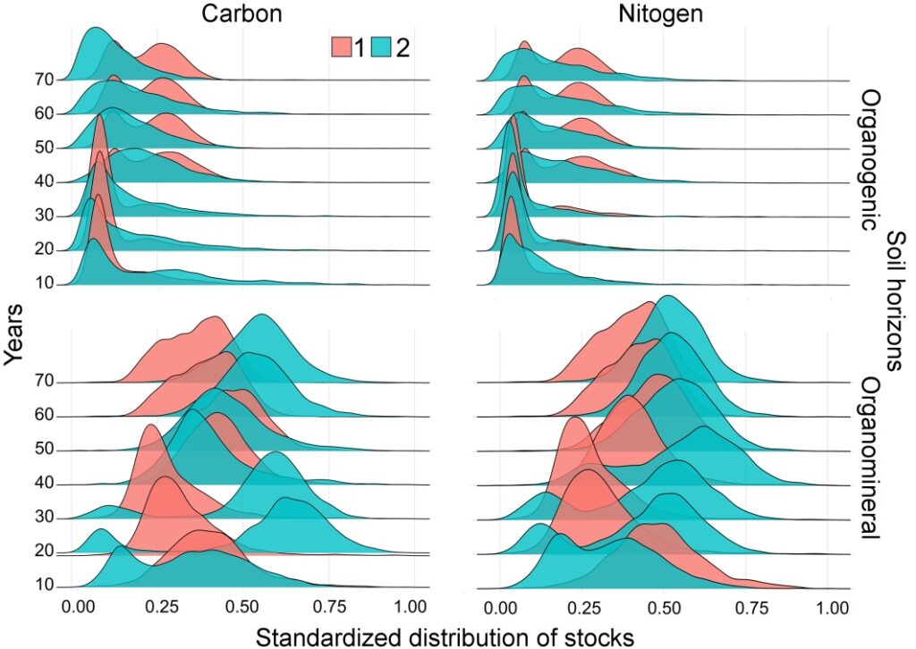
Figure 33. Standardized distribution of C and N stocks in organogenic (forest floor) and organomineral soil horizons in a pine crop scenario with a regular tree arrangement. Symbols are the same as in Fig. 29
These differences are particularly noticeable when analyzing the average OM dynamics in forest floor (Fig. 34), which in this scenario is formed anew after disturbances associated with site preparation for planting forest crops. In real conditions of forest crop establishment such contrast of soil conditions is not observed, which is explained by the role of ground cover plant litter, actively developing in the absence of competition from the stand and richer in nitrogen than pine litter fractions. All this contributes to the formation of a less contrasting picture of the spatial distribution of organic matter and nitrogen reserves in soils.
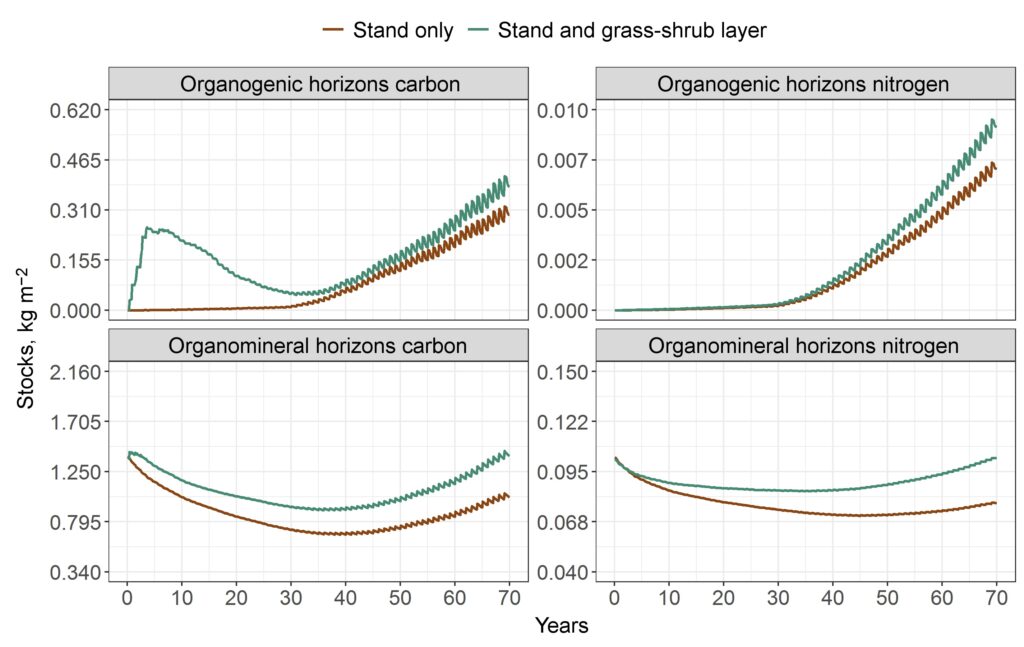
Figure 34. Dynamics of OM and nitrogen stocks distribution in forest floor (organogenic horizons) and organomineral part of soil profile in the scenario of Pinus sylvestris crops with regular planting scheme on sod subsoil: mean values of indicators for corresponding horizons
CONCLUSION
Within the framework of the presented study, the integration of multi-scale simulation models is realized, which consider and reproduce in simulation experiments the hierarchy and spatial heterogeneity of forest ecosystems with a complex structure of subordination and functional interrelationships between their components. The model system is parameterized for forest ecosystems of the European part of Russia, taking into account the range of soil and climatic conditions, diversity and complexity of species composition and spatial structures, which forms a variety of functional ecological relationships. Both previously published studies data and the results of our own experimental studies were used for development of the model system, its parameterization and validation. It should be noted that the importance of spatial dimensions in the study of ecosystem dynamics was stated much later (Watt, 1947) than systematic attempts to describe the dynamics of plant populations began. Until recently, modeling approaches have been limited to biometric quantitative analysis of ecological data. Researchers have rarely set out to comprehensively and exhaustively collect data to build and verify ecosystem-level models.
Most of the currently existing mathematical or computer models of plant communities that reproduce the structure of tree crowns do not take into account the occurrence of crown asymmetry as a result of competition between trees for PAR resources, although the importance of solving such a problem is obvious (Cescatti, 1997a, 1997b). Root competition for soil nutrient elements is also described in a simplified manner in most models, and only a few models are able to describe the distribution of woody plant roots in the soil in relation to competition from neighbors and heterogeneity of soil conditions (Mao et al., 2015; Shanin et al., 2015a). Therefore, most existing models are generally unable to reproduce the rapid responses of root systems to multi-scale environmental changes. Inaccurate estimation of the plasticity of crowns and root systems in models can lead to incorrect estimation of the intensity of competition in different parts of the stand (both overestimation and inaccuracy) and, as a consequence, to errors in the calculation of biomass production of individual trees. The proposed system of models has an adaptive character of the algorithm operation, which allows to reproduce the reduction of the acuteness of competitive interaction between individual trees in a stand due to the plasticity of their crowns and root systems. The proposed approach is a compromise between detailed engineering models that recognize the exact structure of crowns, scattering and re-reflection of light rays, but require a large number of input parameters, and simplified models that represent the forest canopy as several layers and tree crowns as objects with homogeneous internal structure.
The realization of this system of models makes it possible to reproduce in simulation experiments the spatial structure of forest phytocenoses (including the initial stages of stand development) and the associated heterogeneity of soil conditions at different hierarchical levels as a tool to control and predict the dynamics, sustainable functioning and biodiversity of forests under different tendencies of their economic use and natural changes. The system of models interfaces ecophysiological processes of different scales. Detailing of it allows to study the influence of heterogeneities of different genesis on ecological processes and properties of plant community and soil. The developed model system reproduces spatial heterogeneity, which significantly affects the dynamics of biogeocenosis and determines its stable functioning in natural conditions and under external influences (up to a certain intensity threshold). This spatially-explicit process model system is capable of reproducing the dynamics of forest ecosystems, taking into account the species and spatial structure of different vegetation layers and its influence through a system of direct and feedback relationships on the formation of soil patchiness conditions. This allows to significantly improve the understanding of ecosystem processes and their contribution to the maintenance of sustainable forest functioning.
Using the developed model system, the role of adaptation mechanisms in mitigating competition between trees for light and nutrients was evaluated in test simulation experiments. In addition, the influence of stand spatial structure on forest ecosystem services such as carbon runoff and soil fertility maintenance is shown. It has also been shown that resource use efficiency is generally higher in mixed and/or uneven-aged stands compared to single-age and single-species stands, which is also demonstrated by experimental data (Brassard et al., 2011). Modeling results show that the increasing complexity of stand structure (e.g., the complexity of its spatial structure, the vertical structure of the tree stand, and the increase in its species diversity) is reflected in a more spatially complex nature of competition for resources, including more efficient use of available resources. For example, simulation experiments have shown a higher resistance of mixed stands to disturbances of various kinds as a result of this and other mechanisms, such as ecological and cenotic strategies of species and separation of ecological niches, which forms a different response of populations of different species to changes in environmental conditions. As a consequence, at the stand scale, this may increase their resilience, especially when combined with the higher productivity of mixed stands noted above.
Thus, the developed model system, due to the wide range of interrelated ecosystem characteristics realized in it, allows simulation assessments of productivity, biogenic cycling of C and N and dynamics of forest ecosystems, taking into account their characteristic multi-scale spatial-species structure and detailed description of competition processes in the stand. This can be used in predictive assessments of forest management efficiency and other environmental objectives in science-based silviculture and sustainable forestry of the near future.
ACKNOWLEDGEMENTS
The study was financially supported by the Russian Science Foundation (project No. 18-14-00362-P): collection of experimental data, parameterization and validation of the model system, simulation experiments and analysis of their results. The development of the model system was carried out within the framework of the topic 122040500037-6 of the State Assignment of FRC PSCBR RAS. Some stages of studies on the development of individual units of the model system were carried out earlier with the financial support of the Russian Foundation for Basic Research. The concept of the model system is based on the ideas formulated by Dr. of biological sciences A.S. Komarov and Dr. of biological sciences O.G. Chertov. We would like to acknowledge all colleagues who participated in the discussion of the structure of the model system and helped in data collection: Dr. of biological sciences M.V. Bobrovsky (ISSP RAS, a separate subdivision of FRC PSCBR RAS); M.P. Shashkov, Candidate of Biological Sciences N.V. Ivanova, Candidate of Biological Sciences L.G. Khanina and Candidate of Biological Sciences V.E. Smirnov (IMPB RAS, branch of PBC RAS named after M.V. Keldysh); Prof., Doctor of Biological Sciences O.V. Smirnova, corresponding member of RAS N.V. Lukina (CEPF RAS); Prof., Doctor of Biological Sciences K.S. Bobkova, Doctor of Biological Sciences S.V. Zagirova, Candidate of Biological Sciences A.F. Osipov, Candidate of Agricultural Sciences A.V. Manov (IB FRC Komi SC UB RAS); Dr. R. Mäkipäää (Natural Resources Institute Finland — Luke); L.K. Ginzhul; management and staff of the “Kaluzhskie Zaseki” State Nature Reserve, and Prioksko-Terrasny State Nature Biosphere Reserve named after M.A. Zablotsky, a branch of the Russian Forest State Forestry Department.
REFERENCES
Abrazhko M. A., Reakcija tonkih kornej eli na iskljuchenie kornevoj konkurencii sosednih derev’ev (The reaction of thin spruce roots to the exclusion of root competition of neighboring trees), Lesovedenie, 1982, No 6, pp. 41–46.
Alberti G., Candido P., Peressotti A., Turco S., Piussi P., Zerbi G., Aboveground biomass relationships for mixed ash (Fraxinus excelsior L. and Ulmus glabra Hudson) stands in Eastern Prealps of Friuli Venezia Giulia (Italy), Annals of Forest Science, 2005, Vol. 62, No 8, pp. 831–836, DOI: 10.1051/forest:2005089.
Aldea J., Ruiz‑Peinado R., del Río M., Pretzsch H., Heym M., Brazaitis G., Jansons A., Metslaid M., Barbeito I., Bielak K., Granhus A., Holm S.‑O., Nothdurft A., Sitko R., Löf M., Species stratification and weather conditions drive tree growth in Scots pine and Norway spruce mixed stands along Europe, Forest Ecology and Management, 2021, Vol. 481, ID 118697, DOI: 10.1016/j.foreco.2020.118697.
Amichev B. Y., Johnston M., van Rees K. C. J., Hybrid poplar growth in bioenergy production systems: Biomass prediction with a simple process-based model (3PG), Biomass and Bioenergy, 2010, Vol. 34, No 5, pp. 687–702, DOI: 10.1016/j.biombioe.2010.01.012.
Appleby R. F., Davies W. J., A possible evaporation site in the guard cell wall and the influence of leaf structure on the humidity response by stomata of woody plants, Oecologia, 1983, Vol. 56, No 1, pp. 30–40, DOI: 10.1007/BF00378214.
Arhangelskaya T. A., Temperaturnyj rezhim kompleksnogo pochvennogo pokrova (Temperature regime of complex soil cover), Moscow: GEOS, 2012, 282 p.
Arkhangelskaya T. A., Gvozdkova A. A., Thermal diffusivity of peat-sand mixtures, IOP Conference Series: Earth and Environmental Science, 2019, Vol. 368, ID 012005, DOI: 10.1088/1755-1315/368/1/012005.
Arii K., Parrott L., Examining the colonization process of exotic species varying in competitive abilities using a cellular automaton model, Ecological Modelling, 2006, Vol. 199, No 3. pp. 219–228, DOI: 10.1016/j.ecolmodel.2006.05.032.
Aschan G., Wittmann C., Pfanz H., Age-dependent bark photosynthesis of aspen twigs, Trees, 2001, Vol. 15, pp. 431–437, DOI: 10.1007/s004680100120.
Badache M., Eslami‑Nejad P., Ouzzane M., Aidoun Z., Lamarche L., A new modeling approach for improved ground temperature profile determination, Renewable Energy, 2016, Vol. 85, pp. 436–444, DOI: 10.1016/j.renene.2015.06.020.
Badía D., López‑García S., Martí C., Ortíz‑Perpiñá O., Girona‑García A., Casanova‑Gascón J., Burn effects on soil properties associated to heat transfer under contrasting moisture content, Science of the Total Environment, 2017, Vol. 601–602, pp. 1119–1128, DOI: 10.1016/j.scitotenv.2017.05.254.
Balboa‑Murias M. A., Rojo A., Álvarez J. G., Merino A., Carbon and nutrient stocks in mature Quercus robur L. stands in NW Spain, Annals of Forest Science, 2006, Vol. 63, No 5, pp. 557–565, DOI: 10.1051/forest:2006038.
Baldocchi D. D., Law B. E., Anthoni P. M., On measuring and modeling energy fluxes above the floor of a homogeneous and heterogeneous conifer forest, Agricultural and Forest Meteorology, 2000, Vol. 102, No 2–3, pp. 187–206, DOI: 10.1016/S0168-1923(00)00098-8.
Balland V., Pollacco J. A. P., Arp P. A., Modeling soil hydraulic properties for a wide range of soil conditions, Ecological Modelling, 2008, Vol. 219, No 3–4, pp. 300–316, DOI: 10.1016/j.ecolmodel.2008.07.009.
Baneva N. A., Izmenenie massy melkih kornej eli v chistyh drevostojah (Change in mass of small spruce roots in pure stands), Lesovedenie, 1980, No 1, pp. 86–89.
Barbeito I., Dassot M., Bayer D., Collet C., Drössler L., Löf M., del Rio M., Ruiz‑Peinado R., Forrester D. I., Bravo‑Oviedo A., Pretzsch H., Terrestrial laser scanning reveals differences in crown structure of Fagus sylvatica in mixed vs. pure European forests, Forest Ecology and Management, 2017, Vol. 405, pp. 381–390, DOI: 10.1016/j.foreco.2017.09.043.
Bauer G., Schulze E.‑D., Mund M., Nutrient contents and concentrations in relation to growth of Picea abies and Fagus sylvatica along a European transect, Tree Physiology, 1997, Vol. 17, No 12, pp. 777–786, DOI: 10.1093/treephys/17.12.777.
Bayer D., Reischl A., Rötzer T., Pretzsch H., Structural response of black locust (Robinia pseudoacacia L.) and small-leaved lime (Tilia cordata Mill.) to varying urban environments analyzed by terrestrial laser scanning: Implications for ecological functions and services, Urban Forestry & Urban Greening, 2018, Vol. 35, pp. 129–138, DOI: 10.1016/j.ufug.2018.08.011.
Belyazid S., Sverdrup H., Kurz D., Braun S., Exploring ground vegetation change for different deposition scenario and methods of estimating critical loads or biodiversity using ForSAFE‑VEG model in Switzerland and Sweden, Water, Air and Soil Pollution, 2011, Vol. 216, pp. 289–317, DOI: 10.1007/s11270-010-0534-6.
Berger U., Piou C., Schiffers K., Grimm V., Competition among plants: Concepts, individual-based modeling approaches, and a proposal for a future research strategy, Perspectives in Plant Ecology, Evolution and Systematics, 2008, Vol. 9, No 3–4, pp. 121–135, DOI: 10.1016/j.ppees.2007.11.002.
Berlin N. G., Kabanov S. V., Mashtakov D. A., Vertikal’naja struktura nadzemnoj fitomassy dubovyh polezashhitnyh lesnyh polos na juzhnyh chernozjomah stepi pravoberezh’ja Saratovskoj oblasti (Vertical structure of the above-ground phytomass of oak field-protective forest belts on the southern chernozems of the steppe right bank of the Saratov region), Vestnik Altajskogo gosudarstvennogo agrarnogo universiteta, 2015, No 5 (127), pp. 87–94.
Betehtina A. A., Bolshakov V. N., Nekrasova O. A., Radchenko T. A., Malygin M. V., Dergacheva M. I., Samozarastanie zolootvalov: ocenka mikorizoobrazovanija, soderzhanija azota i ugleroda v tonkih kornjah Betula pendula Roth. i Populus tremula L. (Self-overgrowing ash dumps: assessment of mycorrhizal formation, nitrogen and carbon content in the fine roots of Betula pendula Roth. and Populus tremula L.), VII Mezhdunarodnaja nauchno-prakticheskaja konferencija “Jekologicheskaja i tehnosfernaja bezopasnost’ gornopromyshlennyh regionov” (VII International Scientific and Practical Conference “Environmental and Technosphere Safety of Mining and Industrial Regions) “, proceedings, Ekaterinburg, 9 April 2019, executive editor A. I. Semjachkov, Ekaterinburg: Institut jekonomiki UrO RAN, Uralskij gosudarstvennyj gornyj universitet, 2019, pp. 34–39.
Bielak K., Dudzińska M., Pretzsch H., Mixed stands of Scots pine (Pinus sylvestris L.) and Norway spruce [Picea abies (L.) Karst] can be more productive than monocultures. Evidence from over 100 years of observation of long-term experiments, Forest Systems, 2014, Vol. 23, No 3, pp. 573–789, DOI: 10.5424/fs/2014233-06195.
Bobkova K. S., Biologicheskaja produktivnost’ hvojnyh lesov Evropejskogo Severo-Vostoka (Biological productivity of coniferous forests of the European Northeast), Leningrad: Nauka, 1987, 156 p.
Bobkova K. S., Stroenie kornevyh sistem drevesnyh porod v razlichnyh tipah sosnovyh lesov Zelenoborskogo stacionara (The structure of root systems of tree species in various types of pine forests of the Zelenoborsky station), Voprosy jekologii sosnjakov Severa: Trudy Komi filiala AN SSSR (Problems of ecology of pine forests of the North: Proceedings of the Komi branch of the Academy of Sciences of the USSR), 1972, Vol. 24, pp. 52–69.
Bobkova K. S., Galenko J. P., Zagirova S. V., Patov A. I., Sostav i struktura drevostoev korennyh el’nikov predgorij Urala bassejna verhnej Pechory (Composition and structure of native spruce stands in the foothills of the Urals in the Upper Pechora basin), Lesovedenie, 2007, No 3, pp. 23–31.
Bobkova K. S., Urnyshev A. P., Urnyshev V. A., Vertikal’noe raspredelenie fitomassy v elovyh lesah evropejskogo Severo-Vostoka (Vertical distribution of phytomass in spruce forests of the European Northeast), Lesovedenie, 2000, No 3, pp. 49–54.
Bobrovskij M. V., Lesnye pochvy Evropejskoj Rossii (Forest soils of European Russia), Moscow: Tov-vo nauchn. izd. KMK, 2010, 359 p.
Bobrovskij M. V., Lojko S. V., Vozrast i osobennosti genezisa temnogumusovyh pochv “Kaluzhskih zasek” (Age and features of the genesis of dark-humus soils of the “Kaluzhskie zaseki”), Vestnik MGU, Ser. Geogr., 2019, No 5, pp. 108–117.
Bocock K. L., Changes in the amounts of dry matter, nitrogen, carbon and energy in decomposing woodland leaf litter in relation to the activities of the soil fauna, Journal of Ecology, 1964, Vol. 52, No 2, pp. 273–284, DOI: 10.2307/2257595.
Bolte A., Villanueva I., Interspecific competition impacts on the morphology and distribution of fine roots in European beech (Fagus sylvatica L.) and Norway spruce (Picea abies (L.) Karst.), European Journal of Forest Research, 2006, Vol. 125, pp. 15–26, DOI: 10.1007/s10342-005-0075-5.
Bonten L. T. C., Groeneberg J. E., Meesenburg H., De Vries W., Using advanced surface complexation models for modelling soil chemistry under forests: Solling forest, Germany, Environmental Pollution, 2011, Vol. 159, No 10, pp. 2831–2839, DOI: 10.1016/j.envpol.2011.05.002.
Brandtberg P.‑O., Bengtsson J., Lundkvist H., Distributions of the capacity to take up nutrients by Betula spp. and Picea abies in mixed stands, Forest Ecology and Management, 2004, Vol. 198, No 1–3. pp. 193–208, DOI: 10.1016/j.foreco.2004.04.012.
Brassard B. W., Chen H. Y. H., Bergeron Y., Paré D., Differences in fine root productivity between mixed- and single-species stands, Functional Ecology, 2011, Vol. 25, No 1, pp. 238–246, DOI: 10.1111/j.1365-2435.2010.01769.x.
Braun S., Flückiger W., Soil amendments for plantings of urban trees, Soil and Tillage Research, 1998, Vol. 49, No 3, pp. 201–209, DOI: 10.1016/S0167-1987(98)00172-X.
Bréda N., Granier A., Barataud F., Moyne C., Soil water dynamics in an oak stand. I. Soil moisture, water potentials and water uptake by roots, Plant and Soil, 1995, Vol. 172, No 1, pp. 17–27, DOI: 10.1007/BF00020856.
Bristow K. L., Campbell G. S., On the relationship between incoming solar radiation and daily maximum and minimum temperature, Agricultural and Forest Meteorology, 1984, Vol. 31, No 2, pp. 159–166, DOI: 10.1016/0168-1923(84)90017-0.
Brunner A., A light model for spatially explicit forest stand models, Forest Ecology and Management, 1998, Vol. 107, No 1–3, pp. 19–46, DOI: 10.1016/S0378-1127(97)00325-3.
Brunner I., Bakker M. R., Björk R. G., Hirano Y., Lukac M., Aranda X., Børja I., Eldhuset T. D., Helmisaari H.‑S., Jourdan C., Konôpka B., López B. C., Pérez C. M., Persson H., Ostonen I., Fine-root turnover rates of European forests revisited: an analysis of data from sequential coring and ingrowth cores, Plant and Soil, 2013, Vol. 362, pp. 357–372, DOI: 10.1007/s11104-012-1313-5.
Büttner V., Leuschner C., Spatial and temporal patterns of fine root abundance in a mixed oak-beech forest, Forest Ecology and Management, 1994, Vol. 70, No 1–3, pp. 11–21, DOI: 10.1016/0378-1127(94)90071-X.
Campbell G. S., A simple method for determining unsaturated conductivity from moisture retention data, Soil Science, 1974, Vol. 117, No 6, pp. 311–314, DOI: 10.1097/00010694-197406000-00001.
Campbell G. S., Extinction coefficients for radiation in plant canopies calculated using an ellipsoidal inclination angle distribution, Agricultural and Forest Meteorology, 1986, Vol. 36, No 4, pp. 317–321, DOI: 10.1016/0168-1923(86)90010-9.
Campbell G. S., Soil physics with BASIC: transport models for soil–plant systems, Elsevier Science, 1985, 150 p.
Casper B. B., Schenk H. J., Jackson R. B., Defining a plant’s belowground zone of influence, Ecology, 2003, Vol. 84, No 9, pp. 2313–2321, DOI: 10.1890/02-0287.
Cavard X., Bergeron Y., Chen H. Y. H., Paré D., Laganière J., Brassard B., Competition and facilitation between tree species change with stand development, Oikos, 2011, Vol. 120, No 11, pp. 1683–1695, DOI: 10.1111/j.1600-0706.2011.19294.x.
Celniker J. L., Korzuhin M. D., Semenov S. M., Model’nyj analiz shirotnogo raspredelenija produktivnosti lesnyh porod Rossii (Model analysis of the latitudinal distribution of productivity of forest species in Russia), Lesovedenie, 2010, No 2, pp. 36–45.
Celniker J. L., Korzuhin M. D., Suvorova G. G., Jankova L. S., Kopytova L. D., Filippova A. K., Analiz vlijanija faktorov sredy na fotosintez hvojnyh Predbajkal’ja (Analysis of the influence of environmental factors on photosynthesis of coniferous Cisbaikalia), Problemy jekologicheskogo monitoringa i modelirovanija jekosistem, 2007, Vol. 21, pp. 265–292.
Celniker J. L., Malkina I. S., Gurcev A. I., Nikolaev D. K., Kolichestvennaja ocenka svetovogo rezhima po morfostrukturnym pokazateljam kron podrosta eli (Quantitative assessment of the light regime by morphostructural parameters of spruce regrowth crowns), Lesovedenie, 1999, No 4, pp. 64–69.
Cescatti A., Modelling the radiative transfer in discontinuous canopies of asymmetric crowns. I. Model structure and algorithms, Ecological Modelling, 1997a, Vol. 101, No 2–3, pp. 263–274, DOI: 10.1016/S0304-3800(97)00050-1.
Cescatti A., Modelling the radiative transfer in discontinuous canopies of asymmetric crowns. II. Model testing and application in a Norway spruce stand, Ecological Modelling, 1997b, Vol. 101, No 2–3, pp. 275–284, DOI: 10.1016/S0304-3800(97)00055-0.
Chalhoub M., Bernier M., Coquet Y., Philippe M., A simple heat and moisture transfer model to predict ground temperature for shallow ground heat exchangers, Renewable energy, 2017, Vol. 103, pp. 295–307, DOI: 10.1016/j.renene.2016.11.027.
Chenlemuge T., Hertel D., Dulamsuren C., Khishigjargal M., Leuschner C., Hauck M., Extremely low fine root biomass in Larix sibirica forests at the southern drought limit of the boreal forest, Flora, 2013, Vol. 208, No 8–9, pp. 488–496, DOI: 10.1016/j.flora.2013.08.002.
Chertov O. G., Komarov A. S., Tsiplianovsky A. V., A combined simulation model of Scots pine, Norway spruce and Silver birch ecosystems in European boreal zone, Forest Ecology and Management, 1999, Vol. 116, No 1–3, pp. 189–206, DOI: 10.1016/S0378-1127(98)00456-3.
Chertov O. G., Jekologija lesnyh zemel’. Pochvenno-jekologicheskoe issledovanie lesnyh mestoobitanij (Ecology of forest lands. Soil-ecological study of forest habitats), Moscow: Nauka, 1981, 192 p.
Chertov O. G., Komarov A. S., Nadporozhskaya M. A., Bykhovets S. S., Zudin S. L., ROMUL — a model of forest soil organic matter dynamics as a substantial tool for forest ecosystem modelling, Ecological Modelling, 2001, Vol. 138, No 1–3, pp. 289–308, DOI: 10.1016/S0304-3800(00)00409-9.
Chertov O. G., Grabarnik P. Y., Shanin V. N., Bykhovets S. S., Petropavlovskij B. S., Priputina I. V., Frolov P. V., Zubkova E. V., Dinamicheskie modeli nazemnyh jekosistem dlja kolichestvennoj ocenki produktivnosti rastitel’nosti (Dynamic Terrestrial Ecosystem Models for Quantitative Evaluation of Vegetation Productivity), Rastitel’nye resursy, 2019, No 2, pp. 151–169, DOI: 10.1134/S0033994619020031.
Chertov O. G., Komarov A. S., Bykhovets S. S., Bhatti J. S., Razlichie jekologicheskih strategij hvojnyh porod v evropejskih i kanadskih boreal’nyh lesah (Difference in ecological strategies of conifers in European and Canadian boreal forests), Biosfera, 2015, Vol. 7, No 3, pp. 328–337.
Chertov O., Komarov A., Shaw C., Bykhovets S., Frolov P., Shanin V., Grabarnik P., Priputina I., Zubkova E., Shashkov M., Romul_Hum — A model of soil organic matter formation coupling with soil biota activity. II. Parameterisation of the soil food web biota activity, Ecological Modelling, 2017a, Vol. 345, pp. 125–139, DOI: 10.1016/j.ecolmodel.2016.10.024.
Chertov O., Shaw C., Shashkov M., Komarov A., Bykhovets S., Shanin V., Grabarnik P., Frolov P., Kalinina O., Priputina I., Zubkova E., Romul_Hum model of soil organic matter formation coupled with soil biota activity. III. Parameterisation of earthworm activity, Ecological Modelling, 2017b, Vol. 345, pp. 140–149, DOI: 10.1016/j.ecolmodel.2016.06.013.
Chertov O., Kuzyakov Y., Priputina I., Frolov P., Shanin V., Grabarnik P., Modelling the rhizosphere priming effect in combination with soil food webs to quantify interaction between living plant, soil biota and soil organic matter, Plants, 2022, Vol. 11, No 19, ID 2605, DOI: 10.3390/plants11192605.
Chumachenko S. I., Korotkov V. N., Palenova M. M., Politov D. V., Simulation modeling of long-term stand dynamics at different scenarios of forest management for coniferous-broad-leaved forests, Ecological Modelling, 2003, Vol. 170, No 2–3, pp. 345–362, DOI: 10.1016/S0304-3800(03)00238-2.
Collalti A., Perugini L., Santini M., Chiti T., Nolè A., Matteucci G., Valentini R., A process-based model to simulate growth in forests with complex structure: Evaluation and use of 3D‑CMCC forest ecosystem model in a deciduous forest in Central Italy, Ecological Modelling, 2014, Vol. 272, pp. 362–378, DOI: 10.1016/j.ecolmodel.2013.09.016.
Coops N. C., Waring R. H., Law B. E., Assessing the past and future distribution and productivity of ponderosa pine in the Pacific Northwest using a process model, 3‑PG, Ecological Modelling, 2005, Vol. 183, No 1, pp. 107–124, DOI: 10.1016/j.ecolmodel.2004.08.002.
Cosby B. J., Ferrier R. C., Jenkins A., Wright R. F., Modelling the effects of acid deposition: refinements, adjustments and inclusion of nitrogen dynamics in the MAGIC model, Hydrology and Earth System Sciences, 2001, Vol. 5, No 3, pp. 499–517, DOI: 10.5194/hess-5-499-2001.
Cosby B. J., Hornberger G. M., Clapp R. B., Ginn T., A statistical exploration of the relationships of soil moisture characteristics to the physical properties of soils, Water Resources Research, 1984, Vol. 20, No 6, pp. 682–690, DOI: 10.1029/WR020i006p00682.
Dahlhausen J., Biber P., Rötzer T., Uhl E., Pretzsch H., Tree species and their space requirements in six urban environments worldwide, Forests, 2016, Vol. 7, No 6, ID 111, DOI: 10.3390/f7060111.
Daikoku K., Hattori S., Deguchi A., Aoki Y., Miyashita M., Matsumoto K., Akiyama J., Iida S., Toba T., Fujita Y., Ohta T., Influence of evaporation from the forest floor on evapotranspiration from the dry canopy, Hydrological Processes, 2008, Vol. 22, No 20, pp. 4083–4096, DOI: 10.1002/hyp.7010.
Daniels R. F., Burkhart H. E., Clason T. R., A comparison of competition measures for predicting growth of loblolly pine trees, Canadian Journal of Forest Research, 1986, Vol. 16, No 6, pp. 1230–1237, DOI: 10.1139/x86-218.
Danilin I. M., Tselitan I. A., Dynamics of forest ecosystems regenerated on burned and harvested areas in mountain regions of Siberia: Characteristics of biological diversity, structure and productivity, Siberian Journal of Forest Science, 2016, No 6, pp. 60–72, DOI: 10.15372/SJFS20160606.
Dannenmann M., Simon J., Gasche R., Holst J., Naumann P. S., Kögel‑Knabner I., Knicker H., Mayer H., Schloter M., Pena R., Polle A., Rennenberg H., Papen H., Tree girdling provides insight on the role of labile carbon in nitrogen partitioning between soil microorganisms and adult European beech, Soil Biology and Biochemistry, 2009, Vol. 41, No 8, pp. 1622–1631, DOI: 10.1016/j.soilbio.2009.04.024.
Dauer J., Withington J., Oleksyn J., Chorover J., Chadwick O., Reich P., Eissenstat D., A scanner-based approach to soil profile-wall mapping of root distribution, Dendrobiology, 2009, Vol. 62, pp. 35–40.
De Jaegere T., Hein S., Claessens H. A., A review of the characteristics of small-leaved lime (Tilia cordata Mill.) and their implications for silviculture in a changing climate, Forests, 2016, Vol. 7, No 3, ID 56, DOI: 10.3390/f7030056.
Dejneko I. P., Faustova N. M., Jelementnyj i gruppovoj himicheskij sostav kory i drevesiny osiny (Elemental and group chemical composition of aspen bark and wood), Himija rastitel’nogo syr’ja, 2015, No 1, pp. 51–62, DOI: 10.14258/jcprm.201501461.
Dhiedt E., Baeten L., De Smedt P., Jaroszewicz B., Verheyen K., Tree neighbourhood-scale variation in topsoil chemistry depends on species identity effects related to litter quality, European Journal of Forest Research, 2022, Vol. 141, pp. 1163–1176, DOI: 10.1007/s10342-022-01499-9.
Dhungel R., Aiken R., Evett S. R., Colaizzi P. D., Marek G., Moorhead J. E., Baumhardt R. L., Brauer D., Kutikoff S., Lin X., Energy imbalance and evapotranspiration hysteresis under an advective environment: Evidence from lysimeter, eddy covariance, and energy balance modeling, Geophysical Research Letters, 2021, Vol. 48, No 1, ID e2020GL091203, DOI: 10.1029/2020GL091203.
Diaconu D., Wassenberg M., Spiecker H., Variability of European beech wood density as influenced by interactions between tree-ring growth and aspect, Forest Ecosystems, 2016, Vol. 3, ID 6, DOI: 10.1186/s40663-016-0065-8.
Diagnozy i kljuchi vozrastnyh sostojanij lesnyh rastenij. Derev’ja i kustarniki: metodicheskie razrabotki dlja studentov biologicheskih special’nostej. Diagnoses and keys of the age conditions of forest plants. Trees and shrubs: methodological developments for students of biological specialties, Part 1, O. V. Smirnova (ed.), Moscow: Izd-vo “Prometej” MGPI im. V. I. Lenina, 1989, 102 p.
Díaz‑Maroto I. J., Sylvain T., Analysis of physical properties of wood in three species of Galician oaks for the manufacture of wine barrels. Part I: Wood infradensity, Wood Research, 2016, Vol. 61, No 5, pp. 683–695.
Dickinson R. E., Modeling evapotranspiration for three‐dimensional global climate models, Climate Processes and Climate Sensitivity, 1984, Vol. 29. pp. 58–72, DOI: 10.1029/GM029p0058.
Didion M., Frey B., Rogiers N., Thürig E., Validating tree litter decomposition in the Yasso07 carbon model, Ecological Modelling, 2014, Vol. 291, pp. 58–68, DOI: 10.1016/j.ecolmodel.2014.07.028.
Dreyer E., Le Roux X., Montpied P., Daudet F. A., Masson F., Temperature response of leaf photosynthetic capacity in seedlings from seven temperate tree species, Tree Physiology, 2001, Vol. 21, No 4, pp. 223–232, DOI: 10.1093/treephys/21.4.223.
Dulamsuren C., Hauck M., Bader M., Osokhjargal D., Oyungerel S., Nyambayar S., Runge M., Leuschner C., Water relations and photosynthetic performance in Larix sibirica growing in the forest-steppe ecotone of northern Mongolia, Tree Physiology, 2008, Vol. 29, No 1, pp. 99–110, DOI: 10.1093/treephys/tpn008.
Dulamsuren C., Hauck M., Bader M., Oyungerel S., Osokhjargal D., Nyambayar S., Leuschner C., The different strategies of Pinus sylvestris and Larix sibirica to deal with summer drought in a northern Mongolian forest-steppe ecotone suggest a future superiority of pine in a warming climate, Canadian Journal of Forest Research, 2009, Vol. 39, No 12, pp. 2520–2528, DOI: 10.1139/X09-156.
Ďurkovič J., Čaňová I., Priwitzer T., Biroščíková M., Kapral P., Saniga M. Field assessment of photosynthetic characteristics in micropropagated and grafted wych elm (Ulmus glabra Huds.) trees, Plant Cell, Tissue and Organ Culture (PCTOC), 2010, Vol. 101, pp. 221–228, DOI: 10.1007/s11240-010-9680-1.
Dymov A. A., Bobkova K. S., Tuzhilkina V. V., Rakina D. A., Rastitel’nyj opad v korennom el’nike i listvenno-hvojnyh nasazhdenijah (Plant litter in the primary spruce forest and deciduous-coniferous plantations), Izvestija vysshih uchebnyh zavedenij. Lesnoj zhurnal, 2012, No 3, pp. 7–18.
Èermák J., Leaf distribution in large trees and stands of the floodplain forest in southern Moravia, Tree Physiology, 1998, Vol. 18, No 1, pp. 727–737, DOI: 10.1093/treephys/18.11.727.
Elkie P. C., Rempel R. S., Detecting scales of pattern in boreal forest landscapes, Forest Ecology and Management, 2001, Vol. 147, No 2–3, pp. 253–261, DOI: 10.1016/S0378-1127(00)00467-9.
Evnevich T. V., Savikovskij I. A., Raschjot prjamoj solnechnoj radiacii i kojefficienta prozrachnosti atmosfery (Calculation of direct solar radiation and atmospheric transparency coefficient), Meteorologija i gidrologija, 1989, No 5, pp. 106–109.
Evstigneev O. I., Ontogenetic scales of relation of trees to light (on the example of eastern European forests), Russian Journal of Ecosystem Ecology, 2018, Vol. 3, No 3, DOI: 10.21685/2500-0578-2018-3-3.
Evstigneev O. I., Korotkov V. N., Ontogenetic stages of trees: an overview, Russian Journal of Ecosystem Ecology, 2016, Vol. 1, No 2, DOI: 10.21685/2500-0578-2016-2-1.
Fajardo A., Goodburn J. M., Graham J., Spatial patterns of regeneration in managed uneven-aged ponderosa pine/Douglas-fir forests of Western Montana, USA, Forest Ecology and Management, 2006, Vol. 223, No 1, pp. 255–266, DOI: 10.1016/j.foreco.2005.11.022.
Falster D. S., Duursma R. A., Ishihara M. I., Barneche D. R., FitzJohn R. G., Vårhammar A., …, & York R. A., BAAD: a Biomass And Allometry Database for woody plants, Ecology, 2015, Vol. 96, No 5, pp. 1445–1445, DOI: 10.1890/14-1889.1.
Finsterwalder S., Der suldenferner, Zeitschrift des Deutschen und Österreichischen, Alpenvereins, 1887, Vol. 18, pp. 72–89.
Fjodorov S. F., Issledovanie jelementov vodnogo balansa v lesnoj zone Evropejskoj territorii SSSR (Investigation of the elements of the water balance in the forest zone of the European territory of the USSR), Leningrad: Gidrometeoizdat, 1977, 264 p.
Fomin S. V., Generalized Robinson–Schensted–Knuth correspondence, Journal of Mathematical Sciences, 1988, Vol. 41, No 2, pp. 979–991, DOI: 10.1007/BF01247093.
Forrester D. I., Bauhus J., A review of processes behind diversity — Productivity relationships in forest, Current Forestry Reports, 2016, Vol. 2, pp. 45–61, DOI: 10.1007/s40725-016-0031-2.
Forrester D. I., Tachauer I. H. H., Annighoefer P., Barbeito I., Pretzsch H., Ruiz‑Peinado R., Stark H., Vacchiano G., Zlatanov T., Chakraborty T., Saha S., Sileshi G. W., Generalized biomass and leaf area allometric equations for European tree species incorporating stand structure, tree age and climate, Forest Ecology and Management, 2017, Vol. 396, pp. 160–175, DOI: 10.1016/j.foreco.2017.04.011.
Frank A. B., Liebig M. A., Hanson J. D., Soil carbon dioxide fluxes in northern semiarid grasslands, Soil Biology and Biochemistry, 2002, Vol. 34, No 9, pp. 1235–1241, DOI: 10.1016/S0038-0717(02)00062-7.
Friedlingstein P., Fung I., Holland E., John J., Brasseur G., Erickson D., Schimel D., On the contribution of CO2 fertilization to the missing biospheric sink, Global Biogeochemical Cycles, 1995, Vol. 9, No 4, pp. 541–556, DOI: 10.1029/95GB02381.
Frolov P. V., Shanin V. N., Zubkova E. V., Bykhovets S. S., Grabarnik P. Y., CAMPUS‑S — The model of ground layer vegetation populations in forest ecosystems and their contribution to the dynamics of carbon and nitrogen. I. Problem formulation and description of the model, Ecological Modelling, 2020a, Vol. 431, ID 109184, DOI: 10.1016/j.ecolmodel.2020.109184.
Frolov P. V., Zubkova E. V., Shanin V. N., Bykhovets S. S., Mäkipää R., Salemaa M. CAMPUS‑S — The model of ground layer vegetation populations in forest ecosystems and their contribution to the dynamics of carbon and nitrogen, II. Parameterization, validation and simulation experiments, Ecological Modelling, 2020b, Vol. 431, ID 109183, DOI: 10.1016/j.ecolmodel.2020.109183.
Frolov P. V., Zubkova E. V., Komarov A. S., A cellular automata model for a community comprising two plant species of different growth forms, Biology Bulletin of the Russian Academy of Sciences, 2015, Vol. 42, pp. 279–286, DOI: 10.1134/S1062359015040044.
Frolov P., Shanin V., Zubkova E., Salemaa M., Mäkipää R., Grabarnik P., Predicting biomass of bilberry (Vaccinium myrtillus L.) using rank distribution and root-to-shoot ratio models, Plant Ecology, 2022, Vol. 223, No 2, pp. 131–140, DOI: 10.1007/s11258-021-01199-1.
Gale M. R., Grigal D. F., Vertical root distributions of northern tree species in relation to successional status, Canadian Journal of Forest Research, 1987, Vol. 17, No 8, pp. 829–834, DOI: 10.1139/x87-131.
Gardiner E. S., Löf M., O’Brien J. J., Stanturf J. A., Madsen P., Photosynthetic characteristics of Fagus sylvatica and Quercus robur established for stand conversion from Picea abies, Forest Ecology and Management, 2009, Vol. 258, No 5, pp. 868–878, DOI: 10.1016/j.foreco.2009.03.022.
Gebauer T., Water turnover in species-rich and species-poor deciduous forests: xylem sap flow and canopy transpiration: Dissertation, Biodiversity and Ecology Series B, Vol. 4. Göttingen: Georg-August-Universität, 2010, 146 p., DOI: 10.3249/webdoc-2324.
Gerling N. V., Tarasov S. I., Zakonomernosti assimiljacii dioksida ugleroda hvoej pihty sibirskoj v oblasti vysokih intensivnostej fotosinteticheski aktivnoj radiacii (Patterns of carbon dioxide assimilation in Siberian fir needles in the region of high intensities of photosynthetically active radiation), Biodiagnostika sostojanija prirodnyh i prirodno-tehnogennyh sistem: Materialy XVIII Vserossijskoj nauchno-prakticheskoj konferencii c mezhdunarodnym uchastiem (Biodiagnostics of the state of natural and natural-technogenic systems: Proceedings of the XVIII All-Russian scientific and practical conference with international participation), Kirov: Vjatskij gosudarstvennyj universitet, 2020, P. 111.
Geßler A., Keitel C., Kreuzwieser J., Matyssek R., Seiler W., Rennenberg H., Potential risks for European beech (Fagus sylvatica L.) in a changing climate, Trees, 2007, Vol. 21, No 1, pp. 1–11, DOI: 10.1007/s00468-006-0107-x.
Gessler A., Schneider S., von Sengbusch D., Weber P., Hanemann U., Huber C., Rothe A., Kreutzer K., Rennenberg H., Field and laboratory experiments on net uptake of nitrate and ammonium by the roots of spruce (Picea abies) and beech (Fagus sylvatica) trees, New Phytologist, 1998, Vol. 138, No 2, pp. 275–285, DOI: 10.1046/j.1469-8137.1998.00107.x.
Giagli K., Baar J., Fajstavr M., Gryc V., Vavrčík H., Tree-ring width and variation of wood density in Fraxinus excelsior L. and Quercus robur L. growing in floodplain forests, BioResources, 2018, Vol. 13, No 1, pp. 804–819, DOI: 10.15376/biores.13.1.804-819.
Giertych M. J., Karolewski P., Oleksyn J., Carbon allocation in seedlings of deciduous tree species depends on their shade tolerance, Acta Physiologiae Plantarum, 2015, Vol. 37, ID 216, DOI: 10.1007/s11738-015-1965-x.
Ginijatullin R. H., Kulagin A. J., Sostojanie kornevoj sistemy berjozy povisloj (Betula pendula Roth.) v uslovijah Sterlitamakskogo promyshlennogo centra (State of the root system of the silver birch (Betula pendula Roth.) in the conditions of the Sterlitamak industrial center), Vestnik Udmurtskogo universiteta. Serija “Biologija. Nauki o Zemle“, 2012, No 4, pp. 21–28.
Goisser M., Geppert U., Rötzer T., Paya A., Huber A., Kerner R., Bauerle T., Pretzsch H., Pritsch K., Häberle K. H., Matyssek R., Grams T. E. E., Does belowground interaction with Fagus sylvatica increase drought susceptibility of photosynthesis and stem growth in Picea abies?, Forest Ecology and Management, 2016, Vol. 375, pp. 268–278, DOI: 10.1016/j.foreco.2016.05.032.
Goreaud F., Loreau M., Millier C., Spatial structure and the survival of an inferior competitor: a theoretical model of neighbourhood competition in plants, Ecological Modelling, 2002, Vol. 158, No 1–2, pp. 1–19, DOI: 10.1016/S0304-3800(02)00058-3.
Goulden M. L., Daube B. C., Fan S.‑M., Sutton D. J., Bazzaz A., Munger J. W., Wofsy S. C., Physiological response of a black spruce forest to weather, Journal of Geophysical Research: Atmospheres, 1997, Vol. 102, No D24, pp. 28987–28996, DOI: 10.1029/97JD01111.
Grabarnik P. Y., Chertov O. G., Chumachenko S. I., Shanin V. N., Khanina L. G., Bobrovskij M. V., Bykhovets S. S., Frolov P. V., Integracija imitacionnyh modelej dlja kompleksnoj ocenki jekosistemnyh uslug lesov: metodicheskie podhody (Integration of simulation models for the integrated assessment of forest ecosystem services: methodological approaches), Matematicheskaja biologija i bioinformatika, 2019a, Vol. 14, No 2, pp. 488–499, DOI: 10.17537/2019.14.488.
Grabarnik P. Y., Shanin V. N., Chertov O. G., Priputina I. V., Bykhovets S. S., Petropavlovskij B. S., Frolov P. V., Zubkova E. V., Shashkov M. P., Frolova G. G., Modelirovanie dinamiki lesnyh jekosistem kak instrument prognozirovanija i upravlenija lesami (Modeling the dynamics of forest ecosystems as a tool for forecasting and forest management), Lesovedenie, 2019b, No 6, pp. 488–500, DOI: 10.1134/S0024114819030033.
Grime J. P., Plant strategies, vegetation processes, and ecosystem properties. 2nd edition. John Wiley & Son, 2002, 417 p.
Grossi G., Lendvai A., Peretti G., Ranzi R., Snow precipitation measured by gauges: Systematic error estimation and data series correction in the central Italian Alps, Water, 2017, Vol. 9, No 7, ID 461, DOI: 10.3390/w9070461.
Gryc V., Vavrčík H., Gomola Š., Selected properties of European beech (Fagus sylvatica L.), Journal of Forest Science, 2008, Vol. 54, No 9, pp. 418–425, DOI: 10.17221/59/2008-JFS.
Grygoruk D., Root vitality of Fagus sylvatica L., Quercus petraea Liebl. and Acer pseudoplatanus L. in mature mixed forest stand, Folia Forestalia Polonica. Series A — Forestry, 2016, Vol. 58, No 2, pp. 55–61, DOI: 10.1515/ffp-2016-0006.
Gspaltl M., Bauerle W., Binkley D., Sterba H., Leaf area and light use efficiency patterns of Norway spruce under different thinning regimes and age classes, Forest Ecology and Management, 2013, Vol. 288, pp. 49–59, DOI: 10.1016/j.foreco.2011.11.044.
Guerrero‑Ramírez N. R., Mommer L., Freschet G. T., Iversen C. M., McCormack M. L., …, & Weigelt A., Global root traits (GRooT) database, Global Ecology and Biogeography, 2021, Vol. 30, No 1, pp. 25–37, DOI: 10.1111/geb.13179.
Gulbe J. I., Ermolova L. S., Rozhdestvenskij S. G., Utkin A. I., Celniker J. L., Vertikal’noe raspredelenie poverhnosti list’ev i svetovoj rezhim v listvennyh molodnjakah juzhnoj tajgi (Vertical distribution of leaf surface and light regime in deciduous young forests of the southern taiga), Lesovedenie, 1983, No 2, pp. 21–29.
Gupta A. K., Beta distribution / International encyclopedia of statistical science. Lovric M. (ed.). Springer, 2011, pp. 144–145, DOI: 10.1007/978-3-642-04898-2_144.
Haefner J. W., Poole G. C., Dunn P. V., Decker R. T., Edge effects in computer models of spatial competition, Ecological Modelling, 1991, Vol. 56, pp. 221–244, DOI: 10.1016/0304-3800(91)90201-B.
Hagemeier M., Leuschner C., Functional crown architecture of five temperate broadleaf tree species: Vertical gradients in leaf morphology, leaf angle, and leaf area density, Forests, 2019a, Vol. 10, No 3, ID 265, DOI: 10.3390/f10030265.
Hagemeier M., Leuschner C., Leaf and crown optical properties of five early-, mid- and late-successional temperate tree species and their relation to sapling light demand, Forests, 2019b, Vol. 10, No 10, ID 925, DOI: 10.3390/f10100925.
Hamada J., Pétrissans A., Mothe F., Ruelle J., Pétrissans M., Gérardin P., Variations in the natural density of European oak wood affect thermal degradation during thermal modification, Annals of Forest Science, 2016, Vol. 73, No 2, pp. 277–286, DOI: 10.1007/s13595-015-0499-0.
Hanson P. J., Todd D. E., Amthor J. S., A six-year study of sapling and large-tree growth and mortality responses to natural and induced variability in precipitation and throughfall, Tree Physiology, 2001, Vol. 21, No 6, pp. 345–358, DOI: 10.1093/treephys/21.6.345.
Hansson K., Helmisaari H.‑S., Sah S. P., Lange H., Fine root production and turnover of tree and understorey vegetation in Scots pine, silver birch and Norway spruce stands in SW Sweden, Forest Ecology and Management, 2013, Vol. 309, pp. 58–65, DOI: 10.1016/j.foreco.2013.01.022.
Hansson K., Kleja D. B., Kalbitz K., Larsson H., Amounts of carbon mineralised and leached as DOC during decomposition of Norway spruce needles and fine roots, Soil Biology and Biochemistry, 2010, Vol. 42, No 2, pp. 178–185, DOI: 10.1016/j.soilbio.2009.10.013.
Hättenschwiler S., Gasser P., Soil animals alter plant litter diversity effects on decomposition, Proceedings of the National Academy of Sciences, 2005, Vol. 102, No 5, pp. 1519–1524, DOI: 10.1073/pnas.0404977102.
Havron’in A. V., Kretinin V. M., Dubovskaja L. V., Biologicheskaja akkumuljacija pitatel’nyh jelementov v polezashhitnyh lesnyh polosah na obyknovennom chernozeme (Biological accumulation of nutrients in field-protective forest belts on ordinary chernozem), Voprosy lesnoj biogeocenologii, jekologii i ohrany prirody v stepnoj zone. Mezhvuzovskij sbornik. Issue 2. Kujbyshev: Kujbyshevskij gosudarstvennyj universitet, 1977, pp. 42–49.
Helmisaari H.‑S., Derome J., Nöjd P., Kukkola M., Fine root biomass in relation to site and stand characteristics in Norway spruce and Scots pine stands, Tree Physiology, 2007, Vol. 27, No 10, pp. 1493–1504, DOI: 10.1093/treephys/27.10.1493.
Helmisaari H.‑S., Makkonen K., Kellomäki S., Valtonen E., Mälkönen E., Below- and above-ground biomass, production and nitrogen use in Scots pine stands in eastern Finland, Forest Ecology and Management, 2002, Vol. 165, No 1–3, pp. 317–326, DOI: 10.1016/S0378-1127(01)00648-X.
Helmisaari H.‑S., Sah S., Aro L., Fine roots on intensive forest ecosystem monitoring plots FIP4, FIP10 and FIP11 on Olkiluoto island in 2008, Working Report 2009-127. Finnish Forest Research Institute, 2009, 33 p.
Heräjärvi H., Junkkonen R., Wood density and growth rate of European and hybrid aspen in southern Finland, Baltic Forestry, 2006, Vol. 12, No 1, pp. 2–8.
Herben T., Wildová R., Community-level effects of plant traits in a grassland community examined by multispecies model of clonal plant growth, Ecological Modelling, 2012, Vol. 234, pp. 60–69, DOI: 10.1016/j.ecolmodel.2011.06.012.
Hertel C., Leuchner M., Rötzer T., Menzel A., Assessing stand structure of beech and spruce from measured spectral radiation properties and modeled leaf biomass parameters, Agricultural and Forest Meteorology, 2012, Vol. 165, pp. 82–91, DOI: 10.1016/j.agrformet.2012.06.008.
Hinckley T. M., Lassoie J. P., Running S. W., Temporal and spatial variations in the water status of forest trees, Forest Science, 1978, Vol. 24, Suppl. 1, pp. a0001–z0001.
Hirvelä H., Härkönen K., Lempinen R., Salminen O., MELA2016 Reference Manual [in:] Natural resources and bioeconomy studies 2017/7, Natural Resources Institute Finland, Helsinki, 2017, 547 p.
Hobbie S. E., Oleksyn J., Eissenstat D. M., Reich P. B., Fine root decomposition rates do not mirror those of leaf litter among temperate tree species, Oecologia, 2010, Vol. 162, No 2, pp. 505–513, DOI: 10.1007/s00442-009-1479-6.
Horaskina Y. S., Komarov A. S., Bezrukova M. G., Zhijanski M. K., Modelirovanie dinamiki kal’cija v organicheskih gorizontah pochvy (Modeling of calcium dynamics in organic soil horizons), Komp’juternye issledovanija i modelirovanie, 2010, Vol. 2, No 1, pp. 103–110, DOI: 10.20537/2076-7633-2010-2-1-103-110.
Hristopulos D. T., Gaussian random fields [in:] Random fields for spatial data modeling. Advances in geographic information science, Springer, 2020, pp. 245–307, DOI: 10.1007/978-94-024-1918-4_6
Iivonen S., Kaakinen S., Jolkkonen A., Vapaavuori E., Linder S., Influence of long-term nutrient optimization on biomass, carbon, and nitrogen acquisition and allocation in Norway spruce, Canadian Journal of Forest Research, 2006, Vol. 36, No 6, pp. 1563–1571, DOI: 10.1139/x06-035.
IPCC: Climate Change 2013: The physical science basis. Contribution of Working Group I to the Fifth assessment report of the Intergovernmental Panel on Climate Change / Stocker T. F., Qin D., Plattner G.‑K., Tignor M., Allen S. K., Boschung J., Nauels A., Xia Y., Bex V., Midgley P. M. (eds.). Cambridge: Cambridge University Press, 2013, 1535 p.
Isaev A. S., Ovchinnikova T. M., Suhovol’skij V. G., Raspredelenie fitomassy derev’ev i nasazhdenij po frakcijam: model’ konkurencii (Distribution of the phytomass of trees and plantations by fractions: a model of competition), Problemy jekologicheskogo monitoringa i modelirovanija jekosistem, 2007, Vol. 1, pp. 232–250.
Jacovides C. P., Boland J., Asimakopoulos D. N., Kaltsounides N. A., Comparing diffuse radiation models with one predictor for partitioning incident PAR radiation into its diffuse component in the eastern Mediterranean basin, Renewable Energy, 2010, Vol. 35, No 8, pp. 1820–1827, DOI: 10.1016/j.renene.2009.11.015.
Jagodzinski A. M., Ziółkowski J., Warnkowska A., Prais H., Tree age effects on fine root biomass and morphology over chronosequences of Fagus sylvatica, Quercus robur and Alnus glutinosa stands, PLoS ONE, 2016, Vol. 11, No 2, ID e0148668, DOI: 10.1371/journal.pone.0148668.
Jaloviar P., Kucbel S., Vencurik J., Kýpeťová M., Parobeková Z., Pittner J., Saniga M., Sedmáková D., Underplanted silver fir and common beech cause changes in root stratification and morphology in mature spruce stands, Plant Root, 2018, Vol. 12, pp. 21–30, DOI: 10.3117/plantroot.12.21.
Jarmishko V. T., Vertikal’no-frakcionnaja struktura nadzemnoj fitomassy Pinus sylvestris L. na severnom predele rasprostranenija v uslovijah atmosfernogo zagrjaznenija (Vertical-fractional structure of the aboveground phytomass of Pinus sylvestris L. at the northern limit of distribution under conditions of atmospheric pollution), Rastitel’nye resursy, 1999, Vol. 35, No 1, pp. 3–12.
Jarvis P. G., The interpretation of the variations in leaf water potential and stomatal conductance found in canopies in the field, Philosophical Transactions of the Royal Society of London. Series B: Biological Sciences, 1976, Vol. 273, No 927, pp. 593–610, DOI: 10.1098/rstb.1976.0035.
Jia Y., Yu G., Gao Y., He N., Wang Q., Jiao C., Zuo Y., Global inorganic nitrogen dry deposition inferred from ground- and space-based measurements, Nature Scientific Reports, 2016, Vol. 6, ID 19810, DOI: 10.1038/srep19810.
Jiao W., Wang W., Peng C., Lei X., Ruan H., Yang Y., Grabarnik P., Shanin V., Improving a process-based model to simulate forest carbon allocation under varied stand density, Forests, 2022, Vol. 13, No 8, ID 1212, DOI: 10.3390/f13081212.
Jucker T., Fischer F. J., Chave J., Coomes D. A., Caspersen J., …, & Zavala M. A., Tallo: a global tree allometry and crown architecture database, Global Change Biology, 2022, Vol. 28, No 17, pp. 5254–5268, DOI: 10.1111/gcb.16302.
Juutinen A., Ahtikoski A., Mäkipää R., Shanin V., Effect of harvest interval and intensity on the profitability of uneven-aged management of Norway spruce stands, Forestry: An International Journal of Forest Research, 2018, Vol. 91, No 5, pp. 589–602, DOI: 10.1093/forestry/cpy018.
Jyske T., Mäkinen H., Saranpää P., Wood density within Norway spruce stems, Silva Fennica, 2008, Vol. 42, No 3, pp. 439–455, DOI: 10.14214/sf.248.
Kajimoto T., Matsuura Y., Sofronov M. A., Volokitina A. V., Mori S., Osawa A., Abaimov A. P., Above- and belowground biomass and net primary productivity of a Larix gmelinii stand near Tura, central Siberia, Tree Physiology, 1999, Vol. 19, No 12, pp. 815–822, DOI: 10.1093/treephys/19.12.815.
Kalela E. K., Männiköiden ja kuusikoiden juurisuhteista I (On the horizontal roots in pine and spruce stand I), Silva Fennica (Acta Forestalia Fennica), 1949, Vol. 57, No 2, ID 7398, DOI: 10.14214/aff.7398.
Kalela E. K., Mäntysiemenpuiden ja -puustojen juurisuhteista, Silva Fennica (Acta Forestalia Fennica), 1954, Vol. 61, No 28, ID 7440, DOI: 10.14214/aff.7440.
Kalliokoski T., Root system traits of Norway spruce, Scots pine, and silver birch in mixed boreal forests: an analysis of root architecture, morphology, and anatomy: Dissertation. Dissertationes Forestales, 2011, Vol. 121, 67 p.
Kalliokoski T., Nygren P., Sievänen R., Coarse root architecture of three boreal tree species growing in mixed stands, Silva Fennica, 2008, Vol. 42, No 2, pp. 189–210, DOI: 10.14214/sf.252.
Kalliokoski T., Pennanen T., Nygren P., Sievänen R., Helmisaari H.‑S., Belowground interspecific competition in mixed boreal forests: fine root and ectomycorrhiza characteristics along stand developmental stage and soil fertility gradients, Plant and Soil, 2010a, Vol. 330, pp. 73–89, DOI: 10.1007/s11104-009-0177-9.
Kalliokoski T., Sievänen R., Nygren P., Tree roots as self-similar branching structures: axis differentiation and segment tapering in coarse roots of three boreal forest tree species, Trees, 2010b, Vol. 24, pp. 219–236, DOI: 10.1007/s00468-009-0393-1.
Kang S., Kim S., Oh S., Lee D., Predicting spatial and temporal patterns of soil temperature based on topography, surface cover and air temperature, Forest Ecology and Management, 2000, Vol. 136, No 1–3, pp. 173–184, DOI: 10.1016/S0378-1127(99)00290-X.
Kaplina N. F., Kulakova N. J., Fitomassa i zapasy ugleroda i azota v kontrastnyh po produktivnosti nagornyh dubravah juzhnoj lesostepi (Phytomass and stocks of carbon and nitrogen in upland oak forests with contrasting productivity in the southern forest-steppe), Aridnye jekosistemy, 2021, Vol. 27, No 1 (86), pp. 35–42, DOI: 10.24411/1993-3916-2021-10135.
Kärki T., Variation of wood density and shrinkage in European aspen (Populus tremula), Holz als Roh- und Werkstoff, 2001, Vol. 59, No 1–2, pp. 79–84, DOI: 10.1007/s001070050479.
Karmanova I. V., Sudnicina T. N., Il’ina N. A., Prostranstvennaja struktura slozhnyh sosnjakov (Spatial structure of complex pine forests), Moscow: Nauka, 1987, 100 p.
Karpachevskij L. O., Les i lesnye pochvy (Forest and forest soils), Moscow: Lesn. prom-st’, 1981, 264 p.
Karpechko Y. V., Ocenka prostranstvennoj i vremennoj neodnorodnosti zaderzhanija zhidkih osadkov pologom lesa (Estimation of spatial and temporal heterogeneity of liquid precipitation retention by the forest canopy), Lesovedenie, 1997, No 4, pp. 64–70.
Kätterer T., Reichstein M., Andrén O., Lomander A., Temperature dependence of organic matter decomposition: a critical review using literature data analyzed with different models, Biology and fertility of soil, 1998, Vol. 27, No 3, pp. 258–262, DOI: 10.1007/s003740050430.
Kazda M., Salzer J., Reiter I., Photosynthetic capacity in relation to nitrogen in the canopy of a Quercus robur, Fraxinus angustifolia and Tilia cordata flood plain forest, Tree Physiology, 2000, Vol. 20, No 15, pp. 1029–1037, DOI: 10.1093/treephys/20.15.1029.
Kazimirov N. I., Morozova R. M., Biologicheskij krugovorot veshhestv v el’nikah Karelii (Biological circulation of substances in the spruce forests of Karelia), Leningrad: Nauka, 1973, 175 p.
Kellomäki S., Väisänen H., Strandman H., FinnFor: a model for calculating the response of the boreal forest ecosystem to climate changes / Research Note No 6. Faculty of Forestry, University of Joensuu, Finland, 1993, 120 p.
Kelty M. J., The role of species mixtures in plantation forestry, Forest Ecology and Management, 2006, Vol. 233, No 2–3, pp. 195–204, DOI: 10.1016/j.foreco.2006.05.011.
Kharuk V. I., Im S. T., Petrov I. A., Dvinskaya M. L., Fedotova E. V., Ranson K. J., Fir decline and mortality in the southern Siberian Mountains, Regional Environmental Change, 2017, Vol. 17, No 3, pp. 803–812, DOI: 10.1007/s10113-016-1073-5.
Kiaei M., Samariha A., Wood density and shrinkage of Ulmus glabra in northwestern of Iran, American-Eurasian Journal of Agricultural & Environmental Sciences, 2011, Vol. 11, No 2, рр. 257–260.
Klassifikacija i diagnostika pochv Rossii (Classification and diagnostics of Russian soils) G. V. Dobrovolskij (ed.), Smolensk: Ojkumena, 2004, 341 p.
Kloeppel B. D., Abrams M. D., Ecophysiological attributes of the native Acer saccharum and the exotic Acer platanoides in urban oak forests in Pennsylvania, USA, Tree Physiology, 1995, Vol. 15, No 11, pp. 739–746, DOI: 10.1093/treephys/15.11.739.
Köcher P., Gebauer T., Horna V., Leuschner C., Leaf water status and stem xylem flux in relation to soil drought in five temperate broad-leaved tree species with contrasting water use strategies, Annals of Forest Science, 2009, Vol. 66, No 1, ID 101, DOI: 10.1051/forest/2008076.
Kolari P., Pumpanen J., Kulmala L., Ilvesniemi H., Nikinmaa E., Grönholm T., Hari P., Forest floor vegetation plays an important role in photosynthetic production of boreal forests, Forest Ecology and Management, 2006, Vol. 221, No 1–3, pp. 241–248, DOI: 10.1016/j.foreco.2005.10.021.
Kolobov A. N., Modelirovanie prostranstvenno-vremennoj dinamiki drevesnyh soobshhestv Diss. kand. fiz.-mat. nauk (Modeling the spatio-temporal dynamics of tree communities, Candidate’s phys. and math. sci. thesis), Birobidzhan: Institut kompleksnogo analiza regional’nyh problem DVO RAN, 2013, 133 p.
Kolobov A. N., Frisman E. Y., Evaluate the initial spatial structure and heterogeneity of the composition for spruce and larch stands on real data self-thinning of even-aged stands, Ecological Complexity, 2018, Vol. 34, pp. 89–99, DOI: 10.1016/j.ecocom.2017.09.005.
Kolobov A. N., Lonkina E. S., Frisman E. Y., Modelirovanie i analiz gorizontal’noj struktury smeshannyh drevostoev (na primere probnyh ploshhadej zapovednika “Bastak” v Srednem Priamur’e (Modeling and analysis of the horizontal structure of mixed forest stands (on the example of trial plots of the Bastak nature reserve in the Middle Amur region), Sibirskij lesnoj zhurnal, 2015, No 3, pp. 45–56, DOI: 10.15372/SJFS20150305.
Komarov A. S., Prostranstvennye individual’no-orientirovannye modeli lesnyh jekosistem (Spatial individually-oriented models of forest ecosystems), Lesovedenie, 2010, No 2, pp. 60–68.
Komarov A. S., Prostye struktury rastitel’nogo pokrova, ustojchivye k vneshnim narushenijam (Simple canopy structures resistant to external disturbances) [in:] Vzaimodejstvujushhie Markovskie processy i ih primenenie k matematicheskomu modelirovaniju biologicheskih system (Interacting Markov processes and their application to mathematical modeling of biological systems), Puschino: ONTI NCBI AN SSSR, 1982, pp. 136–143.
Komarov A. S., Chertov O. G., Zudin S. L., Nadporozhskaya M. A., Mikhailov A. V., Bykhovets S. S., Zudina E. V., Zoubkova E. V., EFIMOD 2 — the system of simulation models of forest growth and elements cycles in forest ecosystems, Ecological Modelling, 2003a, Vol. 170, No 2–3, pp. 373–392, DOI: 10.1016/S0304-3800(03)00240-0.
Komarov A. S., Ginzhul L. K., Shanin V. N., Bykhovets S. S., Bobkova K. S., Kuznetsov M. A., Manov A. V., Osipov A. F., Pattern of biomass partitioning into fractions of boreal trees, Biology Bulletin of the Russian Academy of Sciences, 2017b, Vol. 44, No 6, pp. 626–633, DOI: 10.1134/S1062359017060061.
Komarov A. S., Khoraskina Y. S., Bykhovets S. S., Bezrukova M. G., Modelling of soil organic matter and elements of soil nutrition dynamics in mineral and organic forest soils: the ROMUL model expansion, Procedia Environmental Sciences, 2012, Vol. 13, pp. 525–534, DOI: 10.1016/j.proenv.2012.01.043.
Komarov A. S., Palenova M. M., Smirnova O. V., The concept of discrete description of plant ontogenesis and cellular automata models of plant populations, Ecological Modeling, 2003b, Vol. 170, No 2, pp. 427–439, DOI: 10.1016/S0304-3800(03)00243-6.
Komarov A. S., Shanin V. N., Comparative analysis of the influence of climate change and nitrogen deposition on carbon sequestration in forest ecosystems in European Russia: simulation modelling approach, Biogeosciences, 2012, Vol. 9, No 11, pp. 4757–4770, DOI: 10.5194/bg-9-4757–2012.
Komarov A., Chertov O., Bykhovets S., Shaw C., Nadporozhskaya M., Frolov P., Shashkov M., Shanin V., Grabarnik P., Priputina I., Zubkova E., Romul_Hum model of soil organic matter formation coupled with soil biota activity. I. Problem formulation, model description, and testing, Ecological Modelling, 2017a, Vol. 345, pp. 113–124, DOI: 10.1016/j.ecolmodel.2016.08.007.
Korennye elovye lesa Severa: bioraznoobrazie, struktura, funkcii (Indigenous spruce forests of the North: biodiversity, structure, functions), K. S. Bobkova, J. P. Galenko (eds.), Saint Petersburg: Nauka, 2006, 337 p.
Korotkov V. N., Novaja paradigma v lesnoj jekologii (A new paradigm in forest ecology), Biologicheskie nauki, 1991, No 8, pp. 7–19.
Korzuhin M. D., Celniker J. L., Analiz rasprostranenija i chistoj pervichnoj produkcii chetyrjoh lesnyh porod derev’ev v Rossii s pomoshh’ju jekofiziologicheskoj modeli (Analysis of distribution and net primary production of four forest tree species in Russia using an ecophysiological model), Problemy jekologicheskogo monitoringa i modelirovanija jekosistem, 2009, Vol. 22, pp. 92–123.
Korzuhin M. D., Celniker J. L., Model’nyj analiz sovremennyh arealov lesnyh drevesnyh porod na territorii Rossii i ih variacij pri vozmozhnyh izmenenijah klimata (Model analysis of modern areas of forest tree species on the territory of Russia and their variations under possible climate changes), Problemy jekologicheskogo monitoringa i modelirovanija jekosistem, 2010, Vol. 23, pp. 249–268.
Korzuhin M. D., Celniker J. L., Semenov S. M., Jekofiziologicheskaja model’ pervichnoj produktivnosti drevesnyh rastenij i ocenki klimaticheskih predelov ih proizrastanija (Ecophysiological model of primary productivity of woody plants and estimation of climatic limits of their growth), Meteorologija i gidrologija, 2008, No 12, pp. 56–69.
Korzuhin M. D., Vygodskaja N. N., Miljukova I. M., Tatarinov F. A., Celniker J. L., Primenenie objedinennoj modeli fotosinteza i ust’ichnoj provodimosti k analizu assimiljacii ugleroda el’ju i listvennicej v lesah Rossii (Application of the combined model of photosynthesis and stomatal conductance to the analysis of carbon assimilation by spruce and larch in Russian forests), Fiziologija rastenij, 2004, Vol. 51, No 3, pp. 341–354.
Korzukhin M. D., Ter‑Mikaelian M. T., An individual-tree-based model of competition for light, Ecological Modelling, 1995, Vol. 79, No 1–3, pp. 221–229, DOI: 10.1016/0304-3800(94)00039-K.
Koshurnikova N., Makhnykina A., Garmash A., Zlenko L., Verkhovets S., Production of phytomass carbon in the dark coniferous forest of the Western Siberia, 18th International Multidisciplinary Scientific Geoconference SGEM 2018 (2–8 July 2018, Albena, Bulgaria). Conference Proceedings, Vol. 18, pp. 885–892, DOI: 10.5593/sgem2018/3.2.
Kuehne C., Kublin E., Pyttel P., Bauhus J., Growth and form of Quercus robur and Fraxinus excelsior respond distinctly different to initial growing space: Results from 24‑year-old Nelder experiments, Journal of Forestry Research, 2013, Vol. 24, pp. 1–14, DOI: 10.1007/s11676-013-0320-6.
Kükenbrink D., Gardi O., Morsdorf F., Thürig E., Schellenberger A., Mathys L., Above-ground biomass references for urban trees from terrestrial laser scanning data, Annals of Botany, 2021, Vol. 128, No 6, pp. 709–724, DOI: 10.1093/aob/mcab002.
Kulha N., Pasanen L., Holmström L., De Grandpré L., Kuuluvainen T., Aakala T., At what scales and why does forest structure vary in naturally dynamic boreal forests? An analysis of forest landscapes on two continents, Ecosystems, 2018, Vol. 22. pp. 709–724, DOI: 10.1007/s10021-018-0297-2.
Kull O., Koppel A., Net photosynthetic response to light intensity of shoots from different crown positions and age in Picea abies (L.) Karst., Scandinavian Journal of Forest Research, 1987, Vol. 2, No 1–4, pp. 157–166, DOI: 10.1080/02827588709382454.
Kutikoff S., Lin X., Evett S. R., Gowda P., Brauer D., Moorhead J., Marek G., Colaizzi P., Aiken R., Xu L., Owensby C., Water vapor density and turbulent fluxes from three generations of infrared gas analyzers, Atmospheric Measurement Techniques, 2021, Vol. 14, No 2, pp. 1253–1266, DOI: 10.5194/amt-14-1253-2021.
Kuuluvainen T., Hokkanen T. J., Järvinen E., Pukkala T., Factors related to seedling growth in a boreal Scots pine stand: a spatial analysis of a vegetation-soil system, Canadian Journal of Forest Research, 1993, Vol. 23, No 10, pp. 2101–2109, DOI: 10.1139/x93-262.
Kuuluvainen T., Syrjänen K., Kalliola R., Structure of a pristine Picea abies forest in Northeastern Europe, Journal of Vegetation Science, 1998, Vol. 9, No 4, pp. 563–574, DOI: 10.2307/3237272.
Kuzyakova I. F., Kuzyakov Y. V., Thomas E., Wirkung des Mikroreliefs auf die räumliche Variabilität des Kohlenstoffgehaltes eines Podzoluvisols in einem Dauerdüngungsversuch (Effect of microrelief on the spatial variability of carbon content of a Podzoluvisol in a long term field trial), Zeitschrift fur Pflanzenernahrung und Bodenkunde, 1997, Vol. 160, No 5, pp. 555–561, DOI: 10.1002/jpln.19971600506.
Laitakari E., Koivun juuristo (The root system of birch [Betula verrucosa and odorata]), Silva Fennica (Acta Forestalia Fennica), 1934, Vol. 41, No 2, ID 7315, DOI: 10.14214/aff.7315.
Laitakari E., Männyn juuristo. Morfologinen tutkimus (The root system of pine [Pinus sylvestris]: a morphological investigation), Silva Fennica (Acta Forestalia Fennica), 1927, Vol. 33, No 1, ID 7210, DOI: 10.14214/aff.7210.
Lal R., Suleimenov M., Stewart B. A., Hansen D. O., Doraiswamy P., Climate change and terrestrial carbon sequestration in Central Asia. CRC Press, 2007, 512 p., DOI: 10.1201/9780203932698.
Landsberg J. J., Waring R. H., A generalised model of forest productivity using simplified concepts of radiation-use efficiency, carbon balance and partitioning, Forest Ecology and Management, 1997, Vol. 95, No 3, pp. 209–228, DOI: 10.1016/S0378-1127(97)00026-1.
Lasch‑Born P., Suckow F., Reyer C. P. O., Gutsch M., Kollas C., Badeck F.‑W., Bugmann H. K. M., Grote R., Fürstenau F., Lindner M., Schaber J., Description and evaluation of the process-based forest model 4C v2.2 at four European forest sites, Geoscientific Model Development, 2020, Vol. 13, No 11, pp. 5311–5343, DOI: 10.5194/gmd-13-5311-2020.
Lashhinskij N. N., Struktura i dinamika sosnovyh lesov Nizhnego Priangar’ja (Structure and dynamics of pine forests in the Lower Angara region), Moscow: Nauka, 1981, 272 p.
Law B. E., Baldocchi D. D., Anthoni P. M., Below-canopy and soil CO2 fluxes in a ponderosa pine forest, Agricultural and Forest Meteorology, 1999, Vol. 94, No 3–4, pp. 171–188, DOI: 10.1016/S0168-1923(99)00019-2.
Le Goff N., Granier A., Ottorini J.‑M., Peiffer M., Biomass increment and carbon balance of ash (Fraxinus excelsior) trees in an experimental stand in northeastern France, Annals of Forest Science, 2004, Vol. 61, No 6, pp. 577–588, DOI: 10.1051/forest:2004053.
Lebedev E. V., Biologicheskaja produktivnost’ duba chereshchatogo na urovne organizma v ontogeneze v Evropejskoj chasti Rossii (Biological productivity of English oak at the level of an organism in ontogeny in the European part of Russia), Lesnoj vestnik, 2013, No 3, pp. 28–33.
Lebedev E. V., Produktivnost’ berjozy beloj na urovne organizma v ontogeneze v evropejskoj chasti Rossii (White birch productivity at the organism level in ontogeny in the European part of Russia), Izvestija Orenburgskogo gosudarstvennogo agrarnogo universiteta, 2012a, No 4 (36), pp. 18–22.
Lebedev E. V., Produktivnost’ fotosinteza i mineral’noe pitanie lipy melkolistnoj na urovne organizma v ontogeneze v srednem Povolzh’e (The productivity of photosynthesis and mineral nutrition of small-leaved linden at the level of the organism in ontogenesis in the middle Volga region), Vestnik RUDN, serija Jekologija i bezopasnost’ zhiznedejatel’nosti, 2012b, No 4, pp. 5–10.
Lebedev S. V., Chumachenko S. I., Poderevnaja model’ dinamiki mnogovidovogo raznovozrastnogo nasazhdenija (PIXTA) (Tree-by-tree model of the dynamics of a multi-species plant of different ages (PIXTA)), Vestnik Moskovskogo gosudarstvennogo universiteta lesa. Lesnoj vestnik, 2011, No 7 (83), pp. 71–78.
Lebedev V. M., Lebedev E. V., Morfologicheskie, funkcional’nye i fiziologicheskie osobennosti aktivnoj chasti kornevoj sistemy lesoobrazujushhih porod Volgo-vjatskogo regiona) Morphological, functional and physiological features of the active part of the root system of forest-forming species of the Volga-Vyatka region), Agrohimija, 2011, No 4, pp. 38–44.
Lebedev V. M., Lebedev E. V., Vzaimosvjaz’ biologicheskoj produktivnosti i poglotitel’noj dejatel’nosti kornej hvojnyh porod v ontogeneze v zone juzhnoj tajgi Rossii (Interrelation of biological productivity and absorptive activity of coniferous roots in ontogeny in the southern taiga zone of Russia), Agrohimija, 2012, No 8, pp. 9–17.
Lehmann J., Kleber M., The contentious nature of soil organic matter, Nature, 2015, Vol. 528, pp. 60–68, DOI: 10.1038/nature16069.
Lemoine D., Peltier J.‑P., Marigo G., Comparative studies of the water relations and the hydraulic characteristics in Fraxinus excelsior, Acer pseudoplatanus and A. opalus trees under soil water contrasted conditions, Annals of Forest Science, 2001, Vol. 58, No 7, pp. 723–731, DOI: 10.1051/forest:2001159.
Leuschner C., Hagemeier M., The economy of canopy space occupation and shade production in early- to late-successional temperate tree species and their relation to productivity, Forests, 2020, Vol. 11, No 3, ID 317, DOI: 10.3390/f11030317.
Leuschner C., Hertel D., Schmid I., Koch O, Muhs A., Hölscher D., Stand fine root biomass and fine root morphology in old-growth beech forests as a function of precipitation and soil fertility, Plant and Soil, 2004, Vol. 258, pp. 43–56, DOI: 10.1023/B:PLSO.0000016508.20173.80.
Levin S. A., The problem of pattern and scale in ecology: the Robert H. MacArthur award lecture, Ecology, 1992, Vol. 73, No 6, pp. 1943–1967, DOI: 10.2307/1941447.
Lexer M. J., Hönninger K., A modified 3D‑patch model for spatially explicit simulation of vegetation composition in heterogeneous landscapes, Forest Ecology and Management, 2001, Vol. 144, No 1–3, pp. 43–65, DOI: 10.1016/S0378-1127(00)00386-8.
Liang W. L., Uchida T., Effects of topography and soil depth on saturated-zone dynamics in steep hillslopes explored using the three-dimensional Richards’ equation, Journal of Hydrology, 2014, Vol. 510, pp. 124–136, DOI: 10.1016/j.jhydrol.2013.12.029.
Liepiņš J., Ivanovs J., Lazdiņš A., Jansons J., Liepiņš K., Mapping of basic density within European aspen stems in Latvia, Silva Fennica, 2017, Vol. 51, No 5, ID 7798, DOI: 10.14214/sf.7798.
Lintunen A., Crown architecture and its role in species interactions in mixed boreal forests: Dissertation. Dissertationes Forestales, Vol. 165, University of Helsinki, Faculty of Agriculture and Forestry, Department of Forest Sciences, 2013, 55 p.
Lintunen A., Kaitaniemi P., Responses of crown architecture in Betula pendula to competition are dependent on the species of neighbouring trees, Trees, 2010, Vol. 24. pp. 411–424, DOI: 10.1007/s00468-010-0409-x.
Lintunen A., Sievänen R., Kaitaniemi P., Perttunen J., Models of 3D crown structure for Scots pine (Pinus sylvestris) and silver birch (Betula pendula) grown in mixed forest, Canadian Journal of Forest Research, 2011, Vol. 41, No 9, pp. 1779–1794, DOI: 10.1139/x11-092.
Loreau M., Separating sampling and other effects in biodiversity experiments, Oikos, 1998, Vol. 82, No 3, pp. 600–602, DOI: 10.2307/3546381.
Lozinov G. L., Osobennosti prostranstvennogo raspredelenija podzemnyh chastej rastenij v lesnyh biogeocenozah Podmoskov’ja (Features of the spatial distribution of underground parts of plants in forest biogeocenoses of the Moscow region), Lesovedenie, 1980, No 1, pp. 58–63.
Lukina N. V., Zapas fitomassy drevostoev sosnjakov lishajnikovyh na severnom predele ih rasprostranenija (Stock of phytomass of lichen pine stands at the northern limit of their distribution), Lesovedenie, 1996, No 3, pp. 28–37.
Lukina N. V., Nikonov V. V., Rajtio H., Himicheskij sostav hvoi sosny na Kol’skom poluostrove (The chemical composition of pine needles on the Kola Peninsula), Lesovedenie, 1994, No 6, pp. 10–21.
Lukina N. V., Orlova M. A., Tikhonova E. V., Tebenkova D. N., Kazakova A. I., Gornov A. V., Smirnov V. E., Knyazeva S. V., Bakhmet O. N., Kryshen A. M., Shashkov M. P., Ershov V. V., The influence of vegetation on the forest soil properties in the republic of Karelia, Eurasian Soil Science, 2019, Vol. 52, No 7, pp. 793–807, DOI: 10.1134/S1064229319050077.
Luk’janec V. B., Soderzhanie azota i zol’nyh jelementov v list’jah duba razlichnogo geograficheskogo proishozhdenija (The content of nitrogen and ash elements in oak leaves of various geographical origin), Lesovedenie, 1980, No 1, pp. 52–57.
Luk’jashhenko K. I., Arhangel’skaja T. A., Modelirovanie temperaturoprovodnosti pochv razlichnogo granulometricheskogo sostava (Modeling the thermal diffusivity of soils of various granulometric composition), Pochvovedenie, 2018, No 2, pp. 179–186, DOI: 10.7868/S0032180X18020053.
Lundegårdh H., Carbon dioxide evolution of soil and crop growth, Soil science, 1927, Vol. 23, No 6, pp. 417–453, DOI: 10.1097/00010694-192706000-00001.
Luoma S., Geographical pattern in photosynthetic light response of Pinus sylvestris in Europe, Functional Ecology, 1997, Vol. 11, No 3, pp. 273–281, DOI: 10.1046/j.1365-2435.1997.00089.x.
Luostarinen K., Tracheid wall thickness and lumen diameter in different axial and radial locations in cultivated Larix sibirica trunks, Silva Fennica, 2012, Vol. 46, No 5, pp. 707–716, DOI: 10.14214/sf.921.
Luostarinen K., Verkasalo E., Birch as sawn timber and in mechanical further processing in Finland. A literature study [in:] Silva Fennica Monographs 1, 2000, 40 p.
Luyssaert S., Schulze E. D., Börner A., Knohl A., Hessenmöller D., Law B. E., Ciais P., Grace J., Old-growth forests as global carbon sinks, Nature, 2008, Vol. 455, pp. 213–215, DOI: 10.1038/nature07276.
Majdi H., Persson H., Spatial distribution of fine roots, rhizosphere and bulk-soil chemistry in an acidified Picea abies stand, Scandinavian Journal of Forest Research, 1993, Vol. 8, No 1–4, pp. 147–155, DOI: 10.1080/02827589309382764.
Mäkelä A., Hari P., Berninger F., Hänninen H., Nikinmaa E., Acclimation of photosynthetic capacity in Scots pine to the annual cycle of temperature, Tree Physiology, 2004, Vol. 24, No 4, pp. 369–376, DOI: 10.1093/treephys/24.4.369.
Mäkelä A., Pulkkinen M., Kolari P., Lagergren F., Berbigier P., Lindroth A., Loustau D., Nikinmaa E., Vesala T., Hari P., Developing an empirical model of stand GPP with the LUE approach: analysis of eddy covariance data at five contrasting conifer sites in Europe, Global Change Biology, 2008, Vol. 14, No 1, pp. 92–108, DOI: 10.1111/j.1365-2486.2007.01463.x.
Mäkelä A., Vanninen P., Vertical structure of Scots pine crowns in different age and size classes, Trees, 2001, Vol. 15, pp. 385–392, DOI: 10.1007/s004680100118.
Mäkinen H., Saranpää P., Linder S., Wood-density variation of Norway spruce in relation to nutrient optimization and fibre dimensions, Canadian Journal of Forest Research, 2002, Vol. 32, No 2, pp. 185–194, DOI: 10.1139/x01-186.
Mao Z., Saint‑André L., Bourrier F., Stokes A., Cordonnier T., Modelling and predicting the spatial distribution of tree root density in heterogeneous forest ecosystems, Annals of Botany, 2015, Vol. 116, No 2, pp. 261–277, DOI: 10.1093/aob/mcv092.
Martens S. N., Breshears D. D., Meyer C. W., Spatial distribution of understory light along the grassland/forest continuum: effects of cover, height, and spatial patterns of tree canopies, Ecological Modelling, 2000, Vol. 126, No 1, pp. 79–93, DOI: 10.1016/S0304-3800(99)00188-X.
Matsinos Y. G., Troumbis A. Y., Modeling competition, dispersal and effects of disturbance in the dynamics of a grassland community using a cellular automaton model, Ecological Modelling, 2002, Vol. 149, No 1–2, pp. 71–83, DOI: 10.1016/S0304-3800(01)00515-4.
Matvienko A. I., Vlijanie azota na mineralizaciju ugleroda v pochvah pod listvennicej sibirskoj i sosnoj obyknovennoj Diss. kand. biol. nauk (Effect of nitrogen on carbon mineralization in soils under Siberian larch and Scots pine. Candidate’s bio. sci. thesis), Krasnojarsk: Institut lesa im. V. N. Sukacheva SO RAN, FIC “Krasnojarskij nauchnyj centr SO RAN”, 2017, 147 p.
Mauer O., Houšková K., Mikita T., The root system of pedunculate oak (Quercus robur L.) at the margins of regenerated stands, Journal of Forest Science, 2017, Vol. 63, No 1, pp. 22–33, DOI: 10.17221/85/2016-JFS.
McCarthy J., Gap dynamics of forest trees: A review with particular attention to boreal forests, Environmental Reviews, 2001, Vol. 9, No 1, pp. 1–59, DOI: 10.1139/a00-012.
Mederski P. S., Bembenek M., Karaszewski Z., Giefing D. F., Sulima‑Olejniczak E., Rosińska M., Łacka A., Density and mechanical properties of Scots pine (Pinus sylvestris L.) wood from a seedling seed orchard, Drewno, 2015, Vol. 58, No 195, pp. 117–124, DOI: 10.12841/wood.1644-3985.123.10.
Medlyn B. E., Dreyer E., Ellsworth D., Forstreuter M., Harley P. C., Kirschbaum M. U. F., Le Roux X., Montpied P., Strassemeyer J., Walcroft A., Wang K., Loustau D., Temperature response of parameters of a biochemically based model of photosynthesis. II. A review of experimental data, Plant, Cell & Environment, 2002, Vol. 25, No 9, pp. 1167–1179, DOI: 10.1046/j.1365-3040.2002.00891.x.
Medvedev I. F., Derevjagin S. S., Kozachenko M. A., Gusakova N. N., Ocenka soderzhanija himicheskih jelementov v drevesine razlichnyh porod derev’ev (Assessment of the content of chemical elements in wood of various tree species), Agrarnyj nauchnyj zhurnal, 2015, No 11, pp. 12–14.
Meier I. C., Knutzen F., Eder L. M., Müller‑Haubold H., Goebel M.‑O., Bachmann J., Hertel D., Leuschner C., The deep root system of Fagus sylvatica on sandy soil: Structure and variation across a precipitation gradient, Ecosystems, 2018, Vol. 21, pp. 280–296, DOI: 10.1007/s10021-017-0148-6.
Meinen C., Hertel D., Leuschner C., Biomass and morphology of fine roots in temperate broad-leaved forests differing in tree species diversity: Is there evidence of below-ground overyielding?, Oecologia, 2009, Vol. 161, pp. 99–111, DOI: 10.1007/s00442-009-1352-7.
Migunova E. S., Lesa i lesnye zemli (kolichestvennaja ocenka vzaimosvjazej) (Forests and forest lands (quantitative assessment of relationships)), Moscow: Ekologija, 1993, 364 p.
Mihalakakou G., Santamouris M., Lewis J. O., Asimakopoulos D. N., On the application of the energy balance equation to predict ground temperature profiles, Solar Energy, 1997, Vol. 60, No 3–4, pp. 181–190, DOI: 10.1016/S0038-092X(97)00012-1.
Miner G. L., Bauerle W. L., Baldocchi D. D., Estimating the sensitivity of stomatal conductance to photosynthesis: a review, Plant, Cell and Environment, 2017, Vol. 40, No 7, pp. 1214–1238, DOI: 10.1111/pce.12871.
Modelirovanie dinamiki organicheskogo veshhestva v lesnyh jekosistemah (Modeling the dynamics of organic matter in forest ecosystems), V. N. Kudeyarov (ed.), Moscow: Nauka, 2007, 380 p.
Moeur M., Spatial models of competition and gap dynamics in old-growth Tsuga heterophylla/Thuja plicata forests, Forest Ecology and Management, 1997, Vol. 94, No 1, pp. 175–186, DOI: 10.1016/S0378-1127(96)03976-X.
Moghaddam E. R., Growth, development and yield in pure and mixed forest stands, International Journal of Advanced Biological and Biomedical Research, 2014, Vol. 2, No 10, pp. 2725–2730.
Molchanov A. A., Poljakova A. F., Harakteristika osnovnyh tipov lesa (Characteristics of the main forest types) [in:] Osnovnye tipy biogeocenozov severnoj tajgi (Main types of biogeocenoses of the northern taiga), Moscow: Nauka, 1977, pp. 44–203.
Molchanov A. A., Poljakova A. F., Produktivnost’ organicheskoj massy v sosnjakah sfagnovyh (Productivity of organic mass in sphagnum pine forests) [in:] Produktivnost’ organicheskoj i biologicheskoj massy lesa (Productivity of organic and biological mass of the forest), Moscow: Nauka, 1974, pp. 43–77.
Montesano P. M., Rosette J., Sun G., North P., Nelson R. F., Dubayah R. O., Ranson K. J., Kharuk V., The uncertainty of biomass estimates from modeled ICESat‑2 returns across a boreal forest gradient, Remote Sensing of Environment, 2015, Vol. 158, pp. 95–109, DOI: 10.1016/j.rse.2014.10.029.
Morozova R. M., Himicheskij sostav rastenij elovyh i berjozovyh lesov Karelii (Chemical composition of plants of spruce and birch forests of Karelia) [in:] Lesnye rastitel’nye resursy Juzhnoj Karelii (Forest plant resources of South Karelia), Petrozavodsk: Karelija, 1971, pp. 57–66.
Morozova R. M., Mineral’nyj sostav rastenij lesov Karelii (Mineral composition of forest plants in Karelia), Petrozavodsk: Goskomizdat, 1991, 100 p.
Mõttus M., Ross J., Sulev M., Experimental study of ratio of PAR to direct integral solar radiation under cloudless conditions, Agricultural and Forest Meteorology, 2001, Vol. 109, No 3, pp. 161–170, DOI: 10.1016/S0168-1923(01)00269-6.
Mõttus M., Sulev M., Baret F., Lopez‑Lozano R., Reinart A., Photosynthetically active radiation: measurement and modeling, [in:] Solar Radiation. Richter C., Lincot D., Gueymard C. A. (Eds.), New York: Springer, 2013, pp. 140–169.
Nabuurs G. J., Schelhaas M. J., Pussinen A., Validation of the European Forest Information Scenario Model (EFISCEN) and a projection of Finnish forests, Silva Fennica, 2000, Vol. 34, No 2, pp. 167–179, DOI: 10.14214/sf.638.
Nahm M., Matzarakis A., Rennenberg H., Geßler A., Seasonal courses of key parameters of nitrogen, carbon and water balance in European beech (Fagus sylvatica L.) grown on four different study sites along a European North-South climate gradient during the 2003 drought, Trees, 2007, Vol. 21, pp. 79–92, DOI: 10.1007/s00468-006-0098-7.
Niinemets Ü., Changes in foliage distribution with relative irradiance and tree size: Differences between the saplings of Acer platanoides and Quercus robur, Ecological Research, 1996, Vol. 11, No 3, pp. 269–281, DOI: 10.1007/BF02347784.
Niinemets Ü., Growth of young trees of Acer platanoides and Quercus robur along a gap-understory continuum: Interrelationships between allometry, biomass partitioning, nitrogen, and shade tolerance, International Journal of Plant Sciences, 1998, Vol. 159, No 2, pp. 318–330, DOI: 10.1086/297553.
Niinemets Ü., Kull O., Stoichiometry of foliar carbon constituents varies along light gradients in temperate woody canopies: Implications for foliage morphological plasticity, Tree Physiology, 1998, Vol. 18, No 7, pp. 467–479, DOI: 10.1093/treephys/18.7.467.
Niinemets Ü., Oja V., Kull O., Shape of leaf photosynthetic electron transport versus temperature response curve is not constant along canopy light gradients in temperate deciduous trees, Plant, Cell & Environment, 1999, Vol. 22, No 12, pp. 1497–1513, DOI: 10.1046/j.1365-3040.1999.00510.x.
Niinemets Ü., Valladares F., Tolerance to shade, drought, and waterlogging of temperate Northern hemisphere trees and shrubs, Ecological Monographs, 2006, Vol. 76, No 4, pp. 521–547, DOI: 10.1890/0012-9615(2006)076[0521:TTSDAW]2.0.CO;2.
Nikonov V. V., Lukina N. V., Smirnova E. V., Isaeva L. G., Vlijanie eli i sosny na formirovanie pervichnoj produktivnosti nizhnimi jarusami hvojnyh lesov Kol’skogo poluostrova (Influence of spruce and pine on the formation of primary productivity by the lower tiers of coniferous forests of the Kola Peninsula), Botanicheskij zhurnal, 2002, Vol. 87, No 8, pp. 112–124.
Nilsson M.‑C., Wardle D. A., Understory vegetation as a forest ecosystem driver: evidence from the northern Swedish boreal forest, Frontiers in Ecology and the Environment, 2005, Vol. 3, No 8, pp. 421–428, DOI: 10.1890/1540-9295(2005)003[0421:UVAAFE]2.0.CO;2.
Nobel P. S., Geller G. N., Temperature modelling of wet and dry desert soils, The Journal of Ecology, 1987, Vol. 75, No 1, pp. 247–258, DOI: 10.2307/2260549.
Norby R. J., DeLucia E. H., Gielen B., Calfapietra C., Giardina C. P., King J. S., Ledford J., McCarthy H. R., Moore D. J. P., Ceulemans R., De Angelis P., Finzi A. C., Karnosky D. F., Kubiske M. E., Lukac M., Pregitzer K. S., Scarascia‑Mugnozza G. E., Schlesinger W. H., Oren R., Forest response to elevated CO2 is conserved across a broad range of productivity, Proceedings of the National Academy of Sciences, 2005, Vol. 102, No 50, pp. 18052–18056, DOI: 10.1073/pnas.0509478102.
Nosova L. M., Osobennosti vertikal’nogo raspredelenija fitomassy lipy raznogo vozrasta v lesnyh biogeocenozah (Peculiarities of vertical distribution of lime phytomass of different ages in forest biogeocenoses), Bjulleten’ Moskovskogo obshhestva ispytatelej prirody. Otdel biologicheskij, 1970, Vol. LXXV(3), pp. 96–107.
Nosova L. M., Holopova L. B., Osobennosti obmena veshhestv mezhdu rastitel’nost’ju i pochvoj v iskusstvennyh nasazhdenijah sosny na dernovo-podzolistyh pochvah (Features of metabolism between vegetation and soil in artificial pine plantations on soddy-podzolic soils) [in:] Obshhie problemy biogeocenologii (General problems of biogeocenology), Moscow: Nauka, 1990, pp. 252–266.
Novickaja J. E., Osobennosti fiziologo-biohimicheskih processov v hvoe i pobegah eli v uslovijah Severa (Features of physiological and biochemical processes in the needles and shoots of spruce in the conditions of the North), Leningrad: Nauka, 1971, 117 p.
Oborny B., Mony C., Herben T., From virtual plants to real communities: a review of modelling clonal growth, Ecological Modelling, 2012, Vol. 23, pp. 3–19, DOI: 10.1016/j.ecolmodel.2012.03.010.
Olchev A., Radler K., Sogachev A., Panferov O., Gravenhorst G., Application of a three-dimensional model for assessing effects of small clear-cuttings on radiation and soil temperature, Ecological Modelling, 2009, Vol. 220, No 21, pp. 3046–3056, DOI: 10.1016/j.ecolmodel.2009.02.004.
Oleksyn J., Żytkowiak R., Reich P. B., Tjoelker M. G., Karolewski P., Ontogenetic patterns of leaf CO2 exchange, morphology and chemistry in Betula pendula trees, Trees, 2000, Vol. 14, pp. 271–281, DOI: 10.1007/PL00009768.
Oostra S., Majdi H., Olsson M., Impact of tree species on soil carbon stocks and soil acidity in southern Sweden, Scandinavian Journal of Forest Research, 2006, Vol. 21, No 5, pp. 364–371, DOI: 10.1080/02827580600950172.
Orlova M. A., Lukina N. V., Kamaev I. O., Smirnov V. E., Kravchenko T. V., Mozaichnost’ lesnyh biogeocenozov i plodorodie pochv (Patchiness nature of forest biogeocenoses and soil fertility), Lesovedenie, 2011, No 6, pp. 39–48.
Oskina N. V., Soderzhanie azota i zol’nyh jelementov v nadzemnoj fitomasse kul’tur sosny obyknovennoj Vladimirskoj, Ul’janovskoj i Kujbyshevskoj oblastej (The content of nitrogen and ash elements in the above-ground phytomass of Scots pine crops in Vladimir, Ulyanovsk and Kuibyshev regions) [in:] Biologicheskaja produktivnost’ lesov Povolzh’ja (Biological productivity of forests of the Volga region), Moscow: Nauka, 1982, pp. 7–11.
Ostonen I., Lõhmus K., Helmisaari H.‑S., Truu J., Meel S., Fine root morphological adaptations in Scots pine, Norway spruce and silver birch along a latitudinal gradient in boreal forests, Tree Physiology, 2007, Vol. 27, No 11, pp. 1627–1634, DOI: 10.1093/treephys/27.11.1627.
Oulehle F., Cosby B. J., Wright R. F., Hruška J., Kapáček J., Krám P., Evans C. D., Moldan F., Modelling soil nitrogen: the MAGIC model with nitrogen retention linked to carbon turnover using decomposer dynamics, Environmental Pollution, 2012, Vol. 165, pp. 158–166, DOI: 10.1016/j.envpol.2012.02.021.
Pace R., De Fino F., Rahman M. A., Pauleit S., Nowak D. J., Grote R., A single tree model to consistently simulate cooling, shading, and pollution uptake of urban trees, International Journal of Biometeorology, 2021, Vol. 65, No 2, pp. 277–289, DOI: 10.1007/s00484-020-02030-8.
Packham J. R., Thomas P. A., Atkinson M. D., Degen T., Biological flora of the British Isles: Fagus sylvatica, Journal of Ecology, 2012, Vol. 100, pp. 1557–1608, DOI: 10.1111/j.1365-2745.2012.02017.x.
Pagès L., Doussan C., Vercambre G., An introduction on below-ground environment and resource acquisition, with special reference on trees. Simulation models should include plant structure and function, Annals of Fores Science, 2000, Vol. 57, No 5–6, pp. 513–520, DOI: 10.1051/forest:2000138.
Pahaut E., Les cristaux de neige et leurs métamorphoses (Snow crystals and their metamorphosies) [in:] Monographies de la Météorologie Nationale 96, 1975, 61 p.
Parajuli A., Nadeau D. F., Anctil F., Parent A. C., Bouchard B., Girard M., Jutras S., Exploring the spatiotemporal variability of the snow water equivalent in a small boreal forest catchment through observation and modeling, Hydrological Processes, 2020, Vol. 34, No 11, pp. 2628–2644, DOI: 10.1002/hyp.13756.
Parton W. J., Stewart J. W. B., Cole C. V., Dynamics of C, N, P and S in grasslands soils: a model, Biogeochemistry, 1988, Vol. 5, pp. 109–131, DOI: 10.1007/BF02180320.
Patankar S., Chislennye metody reshenija zadach teploobmena i dinamiki zhidkosti (Numerical methods for solving problems of heat transfer and fluid dynamics), Moscow: Jenergoatomizdat, 1984, 152 p.
Peichl M., Leava N. A., Kiely G., Above- and belowground ecosystem biomass, carbon and nitrogen allocation in recently afforested grassland and adjacent intensively managed grassland, Plant and Soil, 2012, Vol. 350, pp. 281–296, DOI: 10.1007/s11104-011-0905-9.
Pellicciotti F., Brock B., Strasser U., Burlando P., Funk M., Corripio J., An enhanced temperature-index glacier melt model including the shortwave radiation balance: development and testing for Haut Glacier d’Arolla, Switzerland, Journal of Glaciology, 2005, Vol. 51, No 175, pp. 573–587, DOI: 10.3189/172756505781829124.
Peng C., Liu J., Dang Q., Apps M. J., Jiang H. TRIPLEX: a generic hybrid model for predicting forest growth and carbon and nitrogen dynamic, Ecological Modelling, 2002, Vol. 153, No 1–2, pp. 109–130, DOI: 10.1016/S0304-3800(01)00505-1.
Peñuelas J., Estiarte M., Trends in plant carbon concentration and plant demand for N throughout this century, Oecologia, 1996, Vol. 109, pp. 69–73, DOI: 10.1007/s004420050059.
Persson H., von Fircks Y., Majdi H., Nilsson L. O., Root distribution in a Norway spruce (Picea abies (L.) Karst.) stand subjected to drought and ammonium-sulphate application, Plant and Soil, 1995, Vol. 168, pp. 161–165, DOI: 10.1007/BF00029324.
Perttunen J., The LIGNUM functional-structural tree model: Dissertation. Systems Analysis Laboratory, Helsinki University of Technology, 2009, 52 p.
Petriţan A. M., von Lüpke B., Petriţan I. C., Influence of light availability on growth, leaf morphology and plant architecture of beech (Fagus sylvatica L.), maple (Acer pseudoplatanus L.) and ash (Fraxinus excelsior L.) saplings, European Journal of Forest Research, 2009, Vol. 128, pp. 61–74, DOI: 10.1007/s10342-008-0239-1.
Peuke A. D., Rennenberg H., Carbon, nitrogen, phosphorus, and sulphur concentration and partitioning in beech ecotypes (Fagus sylvatica L.): Phosphorus most affected by drought, Trees, 2004, Vol. 18, No 6, pp. 639–648, DOI: 10.1007/s00468-004-0335-x.
Pigott C. D., Tilia cordata Miller, Journal of Ecology, 1991, Vol. 79, No 4, pp. 1147–1207, DOI: 10.2307/2261105.
Plauborg F., Simple model for 10 cm soil temperature in different soils with short grass, European Journal of Agronomy, 2002, Vol. 17, No 3, pp. 173–179, DOI: 10.1016/S1161-0301(02)00006-0.
Pommerening A., Grabarnik P., Individual-based methods in forest ecology and management, Springer, 2019, 411 p., DOI: 10.1007/978-3-030-24528-3.
Portnov A. M., Bykhovets S. S., Din E. S., Ivanova N. V., Frolov P. V., Shanin V. N., Shashkov M. P., Kolichestvennaja ocenka razmerov okon v pologe starovozrastnogo shirokolistvennogo lesa nazemnymi i distancionnymi metodami (Quantitative assessment of the size of gaps in the canopy of old-growth broad-leaved forest by ground and remote methods), Matematicheskoe modelirovanie v jekologii. Materialy Sed’moj Nacional’noj nauchnoj konferencii s mezhdunarodnym uchastiem (Mathematical modeling in ecology. Proceedings of the Seventh National Scientific Conference with International Participation), 9–12 November 2021, Puschino: FIC PNCBI RAN, 2021, pp. 99–102.
Posch M., Reinds G. J., A very simple dynamic soil acidification model for scenario analyses and target loads calculation, Environmental Modelling and Software, 2009, Vol. 24, No 3, pp. 329–340, DOI: 10.1016/j.envsoft.2008.09.007.
Praciak A., The CABI encyclopedia of forest trees, CABI, 2013, 536 p.
Prentice I. C., Helmisaari H., Silvics of north European trees: Compilation, comparisons and implications for forest succession modelling, Forest Ecology and Management, 1991, Vol. 42, No 1–2, pp. 79–93, DOI: 10.1016/0378-1127(91)90066-5.
Pretzsch H., Canopy space filling and tree crown morphology in mixed-species stands, Forest Ecology and Management, 2014, Vol. 327, pp. 251–264, DOI: 10.1016/j.foreco.2014.04.027.
Pretzsch H., The effect of tree crown allometry on community dynamics in mixed-species stands versus monocultures. A review and perspectives for modeling and silvicultural regulation, Forests, 2019, Vol. 10, No 9, ID 810, DOI: 10.3390/f10090810.
Pretzsch H., Biber P., Ďurský J., The single tree-based stand simulator SILVA: Construction, application and evaluation, Forest Ecology and Management, 2002, Vol. 162, No 1, pp. 3–21, DOI: 10.1016/S0378-1127(02)00047-6.
Pretzsch H., Bielak K., Block J., Bruchwald A., Dieler J., Ehrhart H.‑P., Kohnle U., Nagel J., Spellmann H., Zasada M., Zingg A., Productivity of mixed versus pure stands of oak (Quercus petraea (Matt.) Liebl. and Quercus robur L.) and European beech (Fagus sylvatica L.) along an ecological gradient, European Journal of Forest Research, 2013, Vol. 132, No 2, pp. 263–280, DOI: 10.1007/s10342-012-0673-y.
Pretzsch H., Schütze G., Tree species mixing can increase stand productivity, density and growth efficiency and attenuate the trade-off between density and growth throughout the whole rotation, Annals of Botany, 2021, Vol. 128, No 6, pp. 767–786, DOI: 10.1093/aob/mcab077.
Pretzsch P., Biber P., Uhl E., Dahlhausen J., Rötzer T., Caldentey J., Koike T., van Con T., Chavanne A., Seifert T., du Toit B., Farnden C., Pauleit S., Crown size and growing space requirement of common tree species in urban centres, parks, and forests, Urban Forestry & Urban Greening, 2015, Vol. 14, No 3, pp. 466–479, DOI: 10.1016/j.ufug.2015.04.006.
Priputina I. V., Chertov O. G., Frolov P. V., Shanin V. N., Grabarnik P. Y., Vkljuchenie rizosfernogo prajming-jeffekta v model’ dinamiki organicheskogo veshhestva pochv Romul_Hum: podhody i rezul’taty predvaritel’nogo testirovanija (Inclusion of the rhizospheric priming effect in the Romul_Hum soil organic matter dynamics model: approaches and results of preliminary testing), Matematicheskoe modelirovanie v jekologii. Materialy Sed’moj Nacional’noj nauchnoj konferencii s mezhdunarodnym uchastiem (Mathematical modeling in ecology. Proceedings of the Seventh National Scientific Conference with International Participation), 9–12 November 2021. Puschino: FIC PNCBI RAN, 2021, pp. 106–108.
Priputina I. V., Frolova G. G., Bykhovets S. S., Shanin V. N., Lebedev V. G., Shestibratov K. A., Modelirovanie produktivnosti lesnyh plantacij pri raznyh shemah prostranstvennogo razmeshhenija derev’ev (Modeling the productivity of forest plantations under different tree spatial arrangements), Matematicheskaja biologija i bioinformatika, 2016, Vol. 11, No 2, pp. 245–262, DOI: 10.17537/2016.11.245.
Priputina I. V., Frolova G. G., Shanin V. N., Myakshina T. N., Grabarnik P. Y., Spatial distribution of organic matter and nitrogen in the entic podzols of the Prioksko-Terrasnyi reserve and its relationship with the structure of forest phytocenoses, Eurasian Soil Science, 2020, Vol. 53, No 8, pp. 1021–1032, DOI: 10.1134/S1064229320080128.
Pugachevskij A. B., Cenopopuljacii eli. Struktura, dinamika, faktory reguljacii (Coenopopulations of spruce. Structure, dynamics, factors of regulation), Minsk: Nauka i tehnika, 1992, 206 p.
Puhe J., Growth and development of the root system of Norway spruce (Picea abies) in forest stands — a review, Forest Ecology and Management, 2003, Vol. 175, No 1–3, pp. 253–273, DOI: 10.1016/S0378-1127(02)00134-2.
Pukkala T., Kolström T., A stochastic spatial regeneration model for Pinus sylvestris, Scandinavian Journal of Forest Research, 1992, Vol. 7, No 1–4, pp. 377–385, DOI: 10.1080/02827589209382730.
Pukkala T., Lähde E., Laiho O., Continuous cover forestry in Finland — Recent research results, [in:] Continuous cover Forestry, second ed. Pukkala T., von Gadow K. (eds.) Springer, 2012, pp. 85–128, DOI: 10.1007/978-94-007-2202-6_3.
Püttsepp Ü., Lõhmus K., Persson H. Å., Ahlström K., Fine-root distribution and morphology in an acidic Norway spruce (Picea abies (L.) Karst.) stand in SW Sweden in relation to granulated wood ash application, Forest Ecology and Management, 2006, Vol. 221, No 1–3, pp. 291–298, DOI: 10.1016/j.foreco.2005.10.012.
R Core Team. R: a language and environment for statistical computing. R Foundation for Statistical Computing, 2014, URL: http://www.R-project.org/ (accessed on 31.08.2022).
Rabotnov T. A., Azot v nazemnyh biogeocenozah (Nitrogen in terrestrial biogeocenoses) [in:] Strukturno-funkcional’naja organizacija biogeocenozov (Structural and functional organization of biogeocenoses), Moscow: Nauka, 1980, pp. 69–90.
Räim O., Kaurilind E., Hallik L., Merilo E., Why does needle photosynthesis decline with tree height in Norway spruce?, Plant Biology, 2012, Vol. 14, No 2, pp. 306–314, DOI: 10.1111/j.1438-8677.2011.00503.x.
Rankinen K., Karvonen T., Butterfield D., A simple model for predicting soil temperature in snow-covered and seasonally frozen soil: Model description and testing, Hydrology and Earth System Sciences, 2004, Vol. 8, No 4, pp. 706–716, DOI: 10.5194/hess-8-706-2004.
Ranney T. G., Bir R. E., Skroch W. A., Comparative drought resistance among six species of birch (Betula): influence of mild water stress on water relations and leaf gas exchange, Tree Physiology, 1991, Vol. 8, No 4, pp. 351–360, DOI: 10.1093/treephys/8.4.351.
Rautiainen M., Stenberg P., Simplified tree crown model using standard forest mensuration data for Scots pine, Agricultural and Forest Meteorology, 2005, Vol. 128, No 1–2, pp. 123–129, DOI: 10.1016/j.agrformet.2004.09.002.
Raynaud X., Leadley P. W., Symmetry of belowground competition in a spatially explicit model of nutrient competition, Ecological Modelling, 2005, Vol. 189, pp. 447–453, DOI: 10.1016/j.ecolmodel.2005.03.008.
Remezov N. P., Bykova L. N., Smirnova K. M., Potreblenie i krugovorot azota i zol’nyh jelementov v lesah Evropejskoj chasti SSSR (Consumption and circulation of nitrogen and ash elements in the forests of the European part of the USSR), Moscow: Izdatel’stvo Moskovskogo universiteta, 1959, 284 p.
Remezov N. P., Pogrebnjak P. S., Lesnoe pochvovedenie (Forest soil science), Moscow: Lesnaja promyshlennost’, 1965, 324 p.
Renshaw E., Computer simulation of Sitka spruce: Spatial branching models for canopy growth and root structure, IMA Journal of Mathematics Applied in Medicine & Biology, 1985, Vol. 2, No 3, pp. 183–200, DOI: 10.1093/imammb/2.3.183.
Reshetnikova T. V., Lesnye podstilki kak depo biogennyh jelementov (Forest litter as a depot of biogenic elements), Vestnik Krasnojarskogo gosudarstvennogo agrarnogo universiteta, 2011, No 12, pp. 74–81.
Richards A. E., Forrester D. I., Bauhus J., Scherer‑Lorenzen M., The influence of mixed tree plantations on the nutrition of individual species: a review, Tree Physiology, 2010, Vol. 30, No 9, pp. 1192–1208, DOI: 10.1093/treephys/tpq035.
Romanov E. M., Nureeva T. V., Eremin N. V., The role of planted forests in improving the productive capacity and ecological potential of Scots pine boreal forests in the Middle Volga Region, New Zealand Journal of Forestry Science, 2016, Vol. 46, ID 10, DOI: 10.1186/s40490-016-0066-y.
Ross J. K., Radiacionnyj rezhim i arhitektonika rastitel’nogo pokrova (Radiation regime and architectonics of vegetation cover), Leningrad: Gidrometeoizdat, 1975, 342 p.
Rothe A., Binkley D., Nutritional interactions in mixed species forests: a synthesis, Canadian Journal of Forest Research, 2001, Vol. 31, No 11, pp. 1855–1870, DOI: 10.1139/x01-120.
Rötzer T., Mixing patterns of tree species and their effects on resource allocation and growth in forest stands, Nova Acta Leopoldina, 2013, Vol. 114, No 391, pp. 239–254.
Rötzer T., Liao Y., Goergen K., Schüler G., Pretzsch H., Modelling the impact of climate change on the productivity and water-use efficiency of a central European beech forest, Climate Research, 2013, Vol. 58, No 1, pp. 81–95, DOI: 10.3354/cr01179.
Rusanova G. V., Biologicheskaja produktivnost’ i soderzhanie himicheskih jelementov v fitomasse el’nika-zelenomoshnika (Biological productivity and content of chemical elements in the phytomass of green moss spruce forest) [in:] Produktivnost’ i krugovorot jelementov v fitocenozah severa (Productivity and cycle of elements in phytocenoses of the north), Leningrad: Nauka, 1975, pp. 30–51.
Rust S., Savill P. S., The root systems of Fraxinus excelsior and Fagus sylvatica and their competitive relationships, Forestry: an International Journal of Forest Research, 2000, Vol. 73, No 5, pp. 499–508, DOI: 10.1093/forestry/73.5.499.
Sannikov S. N., Sannikova N. S., Les kak podzemno-somknutaja dendrocenojekosistema (Forest as an underground-closed dendrocenoecosystem), Sibirskij lesnoj zhurnal, 2014, No 1, pp. 25–34.
Saxton K. E., Rawls W. J., Soil water characteristic estimates by texture and organic matter for hydrologic solutions, Soil Science Society of America Journal, 2006, Vol. 70, No 5, pp. 1569–1578, DOI: 10.2136/sssaj2005.0117.
Schaetzl R. J., Knapp B. D., Isard S. A., Modeling soil temperatures and the mesic‐frigid boundary in the central Great Lakes region, 1951–2000, Soil Science Society of America Journal, 2005, Vol. 69, No 6, pp. 2033–2040, DOI: 10.2136/sssaj2004.0349.
Schiffers K., Tielbörger K., Tietjen B., Jeltsch F., Root plasticity buffers competition among plants: theory meets experimental data, Ecology, 2011, Vol. 92, No 3, pp. 610–620, DOI: 10.1890/10-1086.1.
Schmid I., The influence of soil type and interspecific competition on the fine root system of Norway spruce and European beech, Basic and Applied Ecology, 2002, Vol. 3, No 4, pp. 339–346, DOI: 10.1078/1439-1791-00116.
Schmid I., Kazda M., Root distribution of Norway spruce in monospecific and mixed stands on different soils, Forest Ecology and Management, 2002, Vol. 159, No 1–2, pp. 37–47, DOI: 10.1016/S0378-1127(01)00708-3.
Schröter M., Härdtle W., von Oheimb G., Crown plasticity and neighborhood interactions of European beech (Fagus sylvatica L.) in an old-growth forest, European Journal of Forest Research, 2012, Vol. 131, pp. 787–798, DOI: 10.1007/s10342-011-0552-y.
Seidel D., Leuschner C., Müller A., Krause K., Crown plasticity in mixed forests — Quantifying asymmetry as a measure of competition using terrestrial laser scanning, Forest Ecology and Management, 2011, Vol. 261, No 11, pp. 2123–2132, DOI: 10.1016/j.foreco.2011.03.008.
Seidl R., Lexer M. J., Jäger D., Hönninger K., Evaluating the accuracy and generality of a hybrid patch model, Tree Physiology, 2005, Vol. 25, No 7, pp. 939–951, DOI: 10.1093/treephys/25.7.939.
Seidl R., Rammer W., Scheller R. M., Spies T. A., An individual-based process model to simulate landscape-scale forest ecosystem dynamics, Ecological Modelling, 2012, Vol. 231, pp. 87–100, DOI: 10.1016/j.ecolmodel.2012.02.015.
Sekretenko O. P., Analiz prostranstvennoj struktury i jeffektov vzaimodejstvija v biologicheskih soobshhestvah. Avtoref. Diss. k. f.-m. n. (Analysis of the spatial structure and effects of interaction in biological communities Extended abstract of candidate’s phys. and math. sci. thesis), Krasnojarsk, 2001, 22 p.
Shanin V. N., Grabarnik P. Y., Bykhovets S. S., Chertov O. G., Priputina I. V., Shashkov M. P., Ivanova N. V., Stamenov M. N., Frolov P. V., Zubkova E. V., Ruchinskaja E. V., Parametrizacija modeli produkcionnogo processa dlja dominirujushhih vidov derev’ev Evropejskoj chasti RF v zadachah modelirovanija dinamiki lesnyh jekosistem (Parameterization of the production process model for the dominant tree species of the European part of the Russian Federation in the problems of modeling the dynamics of forest ecosystems), Matematicheskaja biologija i bioinformatika, 2019, Vol. 14, No 1, pp. 54–76, DOI: 10.17537/2019.14.54.
Shanin V. N., Grabarnik P. Y., Shashkov M. P., Ivanova N. V., Bykhovets S. S., Frolov P. V., Stamenov M. N., Crown asymmetry and niche segregation as an adaptation of trees to competition for light: conclusions from simulation experiments in mixed boreal stands, Mathematical and Computational Forestry and Natural-Resource Sciences, 2020, Vol. 12, No 1, pp. 26–49, DOI: 10.5281/zenodo.3759256.
Shanin V. N., Rocheva L. K., Shashkov M. P., Ivanova N. V., Moskalenko S. V., Burnasheva E. R., Spatial distribution of root biomass of certain tree species (Picea abies, Pinus sylvestris, Betula sp.), Biology Bulletin of the Russian Academy of Sciences, 2015b, Vol. 42, No 3, pp. 260–268, DOI: 10.1134/S1062359015030115.
Shanin V. N., Shashkov M. P., Ivanova N. V., Bykhovets S. S., Grabarnik P. Y., Issledovanie struktury drevostoev i mikroklimaticheskih uslovij pod pologom lesa na postojannoj probnoj ploshhadi v Prioksko-terrasnom zapovednike (Study of the structure of forest stands and microclimatic conditions under the forest canopy on a permanent sample plot in the Prioksko-Terrasny Reserve), Trudy Prioksko-terrasnogo zapovednika, Issue 7. Moscow: Tovarishhestvo nauchnyh izdanij KMK, 2018, pp. 68–80.
Shanin V. N., Shashkov M. P., Ivanova N. V., Grabarnik P. Y., Vlijanie konkurencii v pologe lesa na prostranstvennuju strukturu drevostoev i formu kron dominantov drevesnogo jarusa na primere lesov evropejskoj chasti Rossii (Influence of competition in the forest canopy on the spatial structure of forest stands and the shape of crowns of tree layer dominants on the example of forests in the European part of Russia), Russian Journal of Ecosystem Ecology, 2016, Vol. 1, No 4, pp. 112–125, DOI: 10.21685/2500-0578-2016-4-5.
Shanin V., Hökkä H., Grabarnik P., Testing the performance of some competition indices against experimental data and outputs of spatially-explicit simulation models, Forests, 2021a, Vol. 12, No 10, ID 1415, DOI: 10.3390/f12101415.
Shanin V., Juutinen A., Ahtikoski A., Frolov P., Chertov O., Rämö J., Lehtonen A., Laiho R., Mäkiranta P., Nieminen M., Laurén A., Sarkkola S., Penttilä T., Ťupek B., Mäkipää R., Simulation modelling of greenhouse gas balance in continuous-cover forestry of Norway spruce stands on nutrient-rich drained peatlands, Forest Ecology and Management, 2021b, Vol. 496, ID 119479, DOI: 10.1016/j.foreco.2021.119479.
Shanin V., Mäkipää R., Shashkov M., Ivanova N., Shestibratov K., Moskalenko S., Rocheva L., Grabarnik P., Bobkova K., Manov A., Osipov A., Burnasheva E., Bezrukova M., New procedure for the simulation of belowground competition can improve the performance of forest simulation models, European Journal of Forest Research, 2015a, Vol. 134, pp. 1055–1074, DOI: 10.1007/s10342-015-0909-8.
Shashkov M. P., Bobrovsky M. V., Shanin V. N., Khanina L. G., Grabarnik P. Y., Stamenov M. N., Ivanova N. V., Data on 30‑year stand dynamics in an old-growth broad-leaved forest in the Kaluzhskie Zaseki State Nature Reserve, Russia, Nature Conservation Research, 2022, Vol. 7, Suppl. 1, pp. 24–37, DOI: 10.24189/ncr.2022.013.
Shein E. V., Kurs fiziki pochv (Course of soil physics), Moscow: Izdatel’stvo MGU, 2005, 432 p.
Shorohova E., Kapitsa E., Influence of the substrate and ecosystem attributes on the decomposition rates of coarse woody debris in European boreal forests, Forest Ecology and Management, 2014, Vol. 315, pp. 173–184, DOI: 10.1016/j.foreco.2013.12.025.
Shugart H. H., Leemans R., Bonan G. B., A system analysis of the global boreal forest. Cambridge University Press, 1992, 580 p., DOI: 10.1017/CBO9780511565489.
Shvidenko A. Z., Schepaschenko D. G., Nil’sson S., Buluj Y. I., Tablicy i modeli rosta i produktivnosti osnovnyh lesoobrazujushhih porod Severnoj Evrazii (normativno-spravochnye materialy) (Tables and models of growth and productivity of the main forest-forming species of Northern Eurasia (normative reference materials)), Moscow: Federal’noe agentstvo lesnogo hozjajstva. Mezhdunarodnyj institut prikladnogo sistemnogo analiza, 2008, 886 p.
Sievänen R., Perttunen J., Nikinmaa E., Kaitaniemi P., Toward extension of a single tree functional-structural model of Scots pine to stand level: Effect of the canopy of randomly distributed, identical trees on development of tree structure, Functional Plant Biology, 2008, Vol. 35, No 10, pp. 964–975, DOI: 10.1071/FP08077.
Sinkkonen A., Red reveals branch die-back in Norway maple Acer platanoides, Annals of Botany, 2008, Vol. 102, No 3, pp. 361–366, DOI: 10.1093/aob/mcn101.
Skarvelis M., Mantanis G., Physical and mechanical properties of beech wood harvested in the Greek public forests, Wood Research, 2013, Vol. 58, No 1, pp. 123–130.
Smejan N. I., Romanova T. A., Turenkov N. I., Tikhonov S. A., Balhanova K. V., Podzolistye pochvy Belorusskoj SSR (Podzolic soils of the Byelorussian SSR) [in:] Podzolistye pochvy zapada Evropejskoj chasti SSSR (Podzolic soils of the west of the European part of the USSR), Moscow: Kolos, 1977, pp. 31–109.
Spielvogel S., Prietzel J., Auerswald K., Kogel‑Knabner I., Site-specific spatial patterns of soil organic carbon stocks in different landscape units of a high-elevation forest including a site with forest dieback, Geoderma, 2009, Vol. 152, No 3–4, pp. 218–230, DOI: 10.1016/j.geoderma.2009.03.009.
Spravochnik po drevesine (Handbook of wood) B. N. Ugolev (ed.), Moscow: Lesnaja promyshlennost’, 1989, 296 p.
Šrámek M., Čermák J., The vertical leaf distribution of Ulmus laevis Pall., Trees, 2012, Vol. 26, pp. 1781–1792, DOI: 10.1007/s00468-012-0747-y.
Stadt K. J., Lieffers V. J., MIXLIGHT: a flexible light transmission model for mixed-species forest stands, Agricultural and Forest Meteorology, 2000, Vol. 102, No 4, pp. 235–252, DOI: 10.1016/S0168-1923(00)00128-3.
Stakanov V. D., Raspredelenie organicheskogo veshhestva v razlichnyh chastjah derev’ev sosny obyknovennoj (Distribution of organic matter in different parts of Scotch pine trees), Lesovedenie, 1990, No 4, pp. 25–33.
Stanley R. P., Differential posets, Journal of the American Mathematical Society, 1988, Vol. 1, No 4, pp. 919–961, DOI: 10.2307/1990995.
Starr M., Helmisaari H.‑S., Merilä P., Modeling rooting depth and distribution from incomplete profile root biomass data, “Roots to the Future”, 8th Symposium of the International Society of Root Research, 26–29 June 2012, Dundee, Scotland, p. 52.
Starr M., Palviainen M., Finér L., Piirainen S., Mannerkoski H., Modelling rooting depth of trees in boreal forests, Abstracts of International Symposium “Root Research and Applications” RootRAP, 2–4 September 2009, Boku Vienna, Austria, 2009, pp. 1–2.
Steffens C., Helfrich M., Joergensen R. G., Eissfeller V., Flessa H., Translocation of 13C‑labeled leaf or root litter carbon of beech (Fagus sylvatica L.) and ash (Fraxinus excelsior L.) during decomposition — a laboratory incubation experiment, Soil Biology and Biochemistry, 2015, Vol. 83, pp. 125–137, DOI: 10.1016/j.soilbio.2015.01.015.
Stoljarov D. P., Polubojarinov V. N., Minaev V. N., Dekatov N. N., Nekrasova G. N., Rekomendacii po ocenke stroenija, tovarnoj struktury i kachestva drevesiny raznovozrastnyh el’nikov s cel’ju organizacii vyborochnogo hozjajstva (Recommendations for assessing the structure, commodity structure and quality of wood of spruce forests of different ages in order to organize a selective economy), Leningrad: NII lesnogo hozjajstva, 1989, 56 p.
Strong W. L., La Roi G. H., Root density — soil relationships in selected boreal forests of central Alberta, Canada, Forest Ecology and Management, 1985, Vol. 12, No 3–4, pp. 233–251, DOI: 10.1016/0378-1127(85)90093-3.
Strous L., Astronomy answers. URL: https://aa.quae.nl/en/index.html (03 October 2022).
Sudachkova N. E., Miljutina I. L., Semenova G. P., Specifika metabolizma listvennicy sibirskoj i listvennicy Gmelina v razlichnyh jekologicheskih uslovijah (Metabolic specifics of Siberian larch and Gmelin larch under different environmental conditions), Hvojnye boreal’noj zony, 2003, Vol. 21, No 1, pp. 54–60.
Sukcessionnye processy v zapovednikah Rossii i problemy sohranenija biologicheskogo raznoobrazija (Succession processes in the reserves of Russia and problems of biological diversity conservation), O. V. Smirnova, E. S. Shaposhnikov (ed.), St. Petersburg: RBO, 1999, 549 p.
Suvorova G., Korzukhin M., Ivanova M., Influence of environmental factors on photosynthesis of three coniferous species, Annual Research & Review in Biology, 2017, Vol. 12, No 3, pp. 1–14, DOI: 10.9734/ARRB/2017/31526.
Sverdrup H., Belyazid S., Nilgard B., Ericson L., Modelling change in ground vegetation response to acid and nitrogen pollution, climate change and forest management, Water, Air & Soil Pollution, 2007, Vol. 7, pp. 163–179, DOI: 10.1007/s11267-006-9067-9.
Swenson J. J., Waring R. H., Fan W., Coops N., Predicting site index with a physiologically based growth model across Oregon, USA, Canadian Journal of Forest Research, 2005, Vol. 35, No 7, pp. 1697–1707, DOI: 10.1139/x05-089.
Tahvanainen T., Forss E., Individual tree models for the crown biomass distribution of Scots pine, Norway spruce and birch in Finland, Forest Ecology and Management, 2008, Vol. 255, No 3–4, pp. 455–467, DOI: 10.1016/j.foreco.2007.09.035.
Tahvonen O., Rämö J., Optimality of continuous cover vs. clear-cut regimes in managing forest resources, Canadian Journal of Forest Research, 2016, Vol. 46, No 7, pp. 891–901, DOI: 10.1139/cjfr-2015-0474.
Takenaka C., Miyahara M., Ohta T., Maximov T. C., Response of larch root development to annual changes of water conditions in Eastern Siberia, Polar Science, 2016, Vol. 10, No 2, pp. 160–166, DOI: 10.1016/j.polar.2016.04.012.
Tanskanen N., Ilvesniemi H., Spatial distribution of fine roots at ploughed Norway spruce forest sites, Silva Fennica, 2007, Vol. 41, No 1, pp. 45–54, DOI: 10.14214/sf.306.
Tardío G., González‑Ollauri A., Mickovski S. B., A non-invasive preferential root distribution analysis methodology from a slope stability approach, Ecological Engineering, 2016, Vol. 97, pp. 46–57, DOI: 10.1016/j.ecoleng.2016.08.005.
Tatarinov F., Urban J., Čermák J., Application of “clump technique” for root system studies of Quercus robur and Fraxinus excelsior, Forest Ecology and Management, 2008, Vol. 255, No 3–4, pp. 495–505, DOI: 10.1016/j.foreco.2007.09.022.
Teichmann J., Ballani F., van den Boogaart K. G., Generalizations of Matérn’s hard-core point processes, Spatial Statistics, 2013, Vol. 3, pp. 33–53, DOI: 10.1016/j.spasta.2013.02.001.
Terehov G. G., Usoltsev V. A., Morfostruktura nasazhdenij i kornenasyshhennost’ rizosfery kul’tur eli sibirskoj i vtorichnogo listvennogo drevostoja na Srednem Urale kak harakteristika ih konkurentnyh otnoshenij (Morphostructure of plantations and root saturation of the rhizosphere of Siberian spruce and secondary deciduous stands in the Middle Urals as a characteristic of their competitive relations), Hvojnye boreal’noj zony, 2010, Vol. XXVII, No 3–4, pp. 330–335.
Thomas F. M., Bögelein R., Werner W., Interaction between Douglas fir and European beech — Investigations in pure and mixed stands, Forstarchiv, 2015, Vol. 86, No 4, pp. 83–91, DOI: 10.4432/0300-4112-86-83.
Thomas F. M., Hartmann G., Tree rooting patterns and soil water relations of healthy and damaged stands of mature oak (Quercus robur L. and Quercus petraea [Matt.] Liebl.), Plant and Soil, 1998, Vol. 203, pp. 145–158, DOI: 10.1023/A:1004305410905.
Thomas P. A., Stone D., La Porta N., Biological flora of the British Isles: Ulmus glabra, Journal of Ecology, 2018, Vol. 106, No 4, pp. 1724–1766, DOI: 10.1111/1365-2745.12994.
Thorpe H. C., Astrup R., Trowbridge A., Coates K. D., Competition and tree crowns: a neighborhood analysis of three boreal tree species, Forest Ecology and Management, 2010, Vol. 259, No 8, pp. 1586–1596, DOI: 10.1016/j.foreco.2010.01.035.
Thurm E. A., Biber P., Pretzsch H., Stem growth is favored at expenses of root growth in mixed stands and humid conditions for Douglas-fir (Pseudotsuga menziesii) and European beech (Fagus sylvatica), Trees, 2017, Vol. 31, No 1, pp. 349–365, DOI: 10.1007/s00468-016-1512-4.
Tikhonova E. V., Tikhonov G. N., Mozaichnost’ hvojno-shirokolistvennyh lesov Valuevskogo lesoparka (Patchiness pattern of coniferous-deciduous forests of the Valuev forest park), Voprosy lesnoj nauki, 2021, Vol. 4, No 3, ID 88, pp. 52–87, DOI: 10.31509/2658-607x- 202143-88.
Toïgo M., Vallet P., Perot T., Bontemps J.‑D., Piedallu C., Courbaud B., Overyielding in mixed forests decreases with site productivity, Journal of Ecology, 2015, Vol. 103, No 2, pp. 502–512, DOI: 10.1111/1365-2745.12353.
Tomczak A., Jelonek T., Jakubowski M., Modulus of elasticity of twin samples (wet and absolute dry) origin from Scots pine (Pinus sylvestris L.) trees broken by wind, Annals of Warsaw University of Life Sciences — SGGW Forestry and Wood Technology, 2011, Vol. 76, pp. 149–153.
Tran Q. T., Tainar D., Safar M., Reverse k nearest neighbor and reverse farthest neighbor search on spatial networks, [in:] Transactions on large-scale data- and knowledge-centered systems, Hameurlain I., Küng J., Wagner R. (eds.), Springer, 2009, pp. 353–372, DOI: 10.1007/978-3-642-03722-1.
Trémolières M., Schnitzler A., Sánchez‑Pérez J.‑M., Schmitt D., Changes in foliar nutrient content and resorption in Fraxinus excelsior L., Ulmus minor Mill. and Clematis vitalba L. after prevention of floods, Annals of Forest Science, 1999, Vol. 56, No 8, pp. 641–650, DOI: 10.1051/forest:19990802.
Tumenbaeva A. R., Sarsekova D. N., Boranbaj Z., Soderzhanie ugleroda v razlichnyh jelementah fitomassy berjozy povisloj (Betula pendula Roth.) v zeljonom pojase goroda Astany (Carbon content in various elements of the phytomass of silver birch (Betula pendula Roth.) in the green belt of the city of Astana), Mezhdunarodnyj nauchno-issledovatel’skij zhurnal, 2018, No 7 (73), pp. 80–84, DOI: 10.23670/IRJ.2018.73.7.016.
Urban J., Čermák J., Ceulemans R., Above- and below-ground biomass, surface and volume, and stored water in a mature Scots pine stand, European Journal of Forest Research, 2015, Vol. 134, pp. 61–74, DOI: 10.1007/s10342-014-0833-3.
Uri V., Kukumägi M., Aosaar J., Varik M., Becker H., Aun K., Krasnova A., Morozov G., Ostonen I., Mander Ü., Lõhmus K., Rosenvald K., Kriiska K., Soosaar K., The carbon balance of a six-year-old Scots pine (Pinus sylvestris L.) ecosystem estimated by different methods, Forest Ecology and Management, 2019, Vol. 433, pp. 248–262, DOI: 10.1016/j.foreco.2018.11.012.
Uri V., Varik M., Aosaar J., Kanal A., Kukumägi M., Lõhmus K., Biomass production and carbon sequestration in a fertile silver birch (Betula pendula Roth) forest chronosequence, Forest Ecology and Management, 2012, Vol. 267, pp. 117–126, DOI: 10.1016/j.foreco.2011.11.033.
Usoltsev V. A., Fitomassa lesov Severnoj Evrazii: normativy i jelementy geografii (Phytomass of forests of Northern Eurasia: standards and elements of geography), Ekaterinburg: UrO RAN, 2002, 762 p.
Usoltsev V. A., Fitomassa model’nyh derev’ev lesoobrazujushhih porod Evrazii: baza dannyh, klimaticheski obuslovlennaja geografija, taksacionnye normativy (Phytomass of model trees of forest-forming species of Eurasia: database, climatically determined geography, taxation standards), Ekaterinburg: Ural’skij gosudarstvennyj lesotehnicheskij universitet, 2016, 336 p.
Usoltsev V. A., Produkcionnye pokazateli i konkurentnye otnoshenija derev’ev. Issledovanie zavisimostej (Production indicators and competitive relations of trees. Dependency research), Ekaterinburg: UGLTU, 2013b, 553 p.
Usoltsev V. A., Vertikal’no-frakcionnaja struktura fitomassy derev’ev. Issledovanie zakonomernostej (Vertical fractional structure of tree phytomass. The study of patterns), Ekaterinburg: UGLTU, 2013a, 603 p.
Utkin A. I., Ermolova L. S., Utkina I. A., Ploshhad’ poverhnosti lesnyh rastenij: sushhnost’, parametry, ispol’zovanie (Surface area of forest plants: essence, parameters, use), Moscow: Nauka, 2008, 292 p.
Vakurov A. D., Poljakova A. F., Krugovorot azota i mineral’nyh jelementov v nizkoproduktivnyh el’nikah severnoj tajgi (Cycle of nitrogen and mineral elements in low-productive spruce forests of the northern taiga), [in:] Krugovorot himicheskih veshhestv v lesu (Cycle of chemicals in the forest), Moscow: Nauka, 1982a, pp. 20–43.
Vakurov D. A., Poljakova A. F., Krugovorot azota i mineral’nyh jelementov v 35‑letnem osinnike (Cycle of nitrogen and mineral elements in a 35‑year-old aspen forest) [in:] Krugovorot himicheskih veshhestv v lesu (Cycle of chemicals in the forest), Moscow: Nauka, 1982b, pp. 44–54.
van der Hage J. C. H., The horizontal component of solar radiation, Agricultural and Forest Meteorology, 1993, Vol. 67, No 1–2, pp. 79–93, DOI: 10.1016/0168-1923(93)90051-I.
Vergarechea M., del Río M., Gordo J., Martín R., Cubero D., Calama R., Spatio-temporal variation of natural regeneration in Pinus pinea and Pinus pinaster Mediterranean forests in Spain, European Journal of Forest Research, 2019, Vol. 138, pp. 313–326, DOI: 10.1007/s10342-019-01172-8.
Verholanceva L. A., Bobkova K. S., Vlijanie pochvennyh uslovij na kornevye sistemy drevesnyh porod v elovyh nasazhdenijah podzony severnoj tajgi (Influence of soil conditions on the root systems of tree species in spruce plantations of the northern taiga subzone), Syktyvkar, 1972, 56 p.
Veselkin D. V., Distribution of fine roots of coniferous trees over the soil profile under conditions of pollution by emissions from a copper-smelting plant, Russian Journal of Ecology, 2002, Vol. 33, No 4, pp. 231–234, DOI: 10.1023/A:1016208118629.
Vesterdal L., Schmidt I. K., Callesen I., Nilsson L. O., Gundersen P., Carbon and nitrogen in forest floor and mineral soil under six common European tree species, Forest Ecology and Management, 2008, Vol. 255, No 1, pp. 35–48, DOI: 10.1016/j.foreco.2007.08.015.
Viherä‑Aarnio A., Velling P., Growth, wood density and bark thickness of silver birch originating from the Baltic countries and Finland in two Finnish provenance trials, Silva Fennica, 2017, Vol. 51, No 4, ID 7731, DOI: 10.14214/sf.7731.
Vinokurova R. I., Lobanova O. V., Specifichnost’ raspredelenija makrojelementov v organah drevesnyh rastenij elovo-pihtovyh lesov Respubliki Marij El (The specificity of the distribution of macroelements in the organs of woody plants of the spruce-fir forests of the Republic of Mari El), Vestnik Povolzhskogo gosudarstvennogo tehnologicheskogo universiteta. Serija: Les. Jekologija. Prirodopol’zovanie, 2011, No 2, pp. 76–83.
von der Heide‑Spravka K. G., Watson G. W., Directional differences in little-leaf linden (Tilia cordata Mill.) crown development, Arboricultural Journal, 1992, Vol. 16, No 3, pp. 243–252, DOI: 10.1080/03071375.1992.9746922.
Vostochnoevropejskie lesa: istorija v golocene i sovremennost’ (Eastern European forests: history in the Holocene and present), Book. 1, O. V. Smirnova (ed.), Moscow: Nauka, 2004, 479 p.
Vtorova V. N., Osobennosti vertikal’nogo raspredelenija himicheskogo sostava strukturnyh komponentov eli i sosny v Podmoskov’e (Features of the vertical distribution of the chemical composition of the structural components of spruce and pine in the Moscow region) [in:] Kompleksnye biogeocenoticheskie issledovanija v lesah Podmoskov’ja (Comprehensive biogeocenotic research in the forests of the Moscow region), Moscow: Nauka, 1982, pp. 5–20.
Wambsganss J., Beyer F., Freschet G. T., Scherer‑Lorenzen M., Bauhus J., Tree species mixing reduces biomass but increases length of absorptive fine roots in European forests, Journal of Ecology, 2021, Vol. 109, No 7, pp. 2678–2691, DOI: 10.1111/1365-2745.13675.
Wang W., Peng C., Zhang S. Y., Zhou X., Larocque G. R., Kneeshaw D. D., Lei X. Development of TRIPLEX-Management model for simulating the response of forest growth to pre-commercial thinning, Ecological Modelling, 2011, Vol. 222, No 14, pp. 2249–2261, DOI: 10.1016/j.ecolmodel.2010.09.019.
Watt A. S., Pattern and process in the plant community, Journal of Ecology, 1947, Vol. 35, No 1/2, pp. 1–22, DOI: 10.2307/2256497.
Way D. A., Domec J.‑C., Jackson R. B., Elevated growth temperatures alter hydraulic characteristics in trembling aspen (Populus tremuloides) seedlings: Implications for tree drought tolerance, Plant, Cell & Environment, 2013, Vol. 36, No 1, pp. 103–115, DOI: 10.1111/j.1365-3040.2012.02557.x.
Weemstra M., Sterck F. J., Visser E. J. W., Kuyper T. W., Goudzwaard L., Mommer L., Fine-root trait plasticity of beech (Fagus sylvatica) and spruce (Picea abies) forests on two contrasting soils, Plant and Soil, 2017, Vol. 415, No 1–2, pp. 175–188, DOI: 10.1007/s11104-016-3148-y.
Widlowski J.‑L., Verstraete M., Pinty B., Gobron N., Allometric relationships of selected European tree species. Technical Report EUR 20855 EN. EC Joint Research Centre, 2003, 61 p.
Wiegand T., Martínez I., Huth A., Recruitment in tropical tree species: revealing complex spatial patterns, The American Naturalist, 2009, Vol. 174, No 4, pp. E106–E140, DOI: 10.1086/605368.
Williams T. G., Flanagan L. B., Effect of changes in water content on photosynthesis, transpiration and discrimination against 13CO2 and C18O16O in Pleurozium and Sphagnum, Oecologia, 1996, Vol. 108, No 1, pp. 38–46, DOI: 10.1007/BF00333212.
Withington J. M., Reich P. B., Oleksyn J., Eissenstat D. M., Comparisons of structure and life span in roots and leaves among temperate trees, Ecological Monographs, 2006, Vol. 76, No 3, pp. 381–397, DOI: 10.1890/0012-9615(2006)076[0381:COSALS]2.0.CO;2.
WRB, 2015, World Reference Base for Soil Resources 2014, update 2015. International soil classification system for naming soils and creating legends for soil maps. World Soil Resources Reports No 106, FAO, Rome.
Wullschleger S. D., Hanson P. J., Sensitivity of sapling and mature-tree water use to altered precipitation regimes, [in:] North American temperate deciduous forest responses to changing precipitation regimes. Hanson P. J., Wullschleger S. D. (eds.), Springer, 2003, pp. 87–98, DOI: 10.1007/978-1-4613-0021-2.
Yastrebov A. B., Different types of heterogeneity and plant competition in monospecific stands, Oikos, 1996, Vol. 75, No 1, pp. 89–97, DOI: 10.2307/3546325.
Yen Y. C., Effective thermal conductivity of ventilated snow, Journal of Geophysical Research, 1962, Vol. 67, No 3, pp. 1091–1098, DOI: 10.1029/JZ067i003p01091.
Yen Y. C., Review of thermal properties of snow, ice, and sea ice. Cold Regions Research and Engineering Laboratory, Report 81‑10. US Army, Corps of Engineers, 1981, 35 p.
Yu X., Wu Z., Jiang W., Guo X., Predicting daily photosynthetically active radiation from global solar radiation in the Contiguous United States, Energy Conversion and Management, 2015, Vol. 89, pp. 71–82, DOI: 10.1016/j.enconman.2014.09.038.
Yuan Z. Y., Chen H. Y. H., Fine root biomass, production, turnover rates, and nutrient contents in boreal forest ecosystems in relation to species, climate, fertility, and stand age: literature review and meta-analyses, Critical Reviews in Plant Sciences, 2010, Vol. 29, No 4, pp. 204–221, DOI: 10.1080/07352689.2010.483579.
Zadworny M., McCormack M. L., Rawlik K., Jagodziński A. M., Seasonal variation in chemistry, but not morphology, in roots of Quercus robur growing in different soil types, Tree Physiology, 2015, Vol. 35, No 6, pp. 644–652, DOI: 10.1093/treephys/tpv018.
Zagirova S. V., Structure and CO2 exchange in the needles of Pinus sylvestris and Abies sibirica, Russian Journal of Plant Physiology, 2001, Vol. 48, No 1, pp. 23–28, DOI: 10.1023/A:1009086211938.
Zajączkowska U., Kozakiewicz P., Interaction between secondary phloem and xylem in gravitropic reaction of lateral branches of Tilia cordata Mill. trees, Holzforschung, 2016, Vol. 70, No 10, pp. 993–1002, DOI: 10.1515/hf-2015-0230.
Zhang C., Stratopoulos L. M. F., Pretzsch H., Rötzer T., How do Tilia cordata Greenspire trees cope with drought stress regarding their biomass allocation and ecosystem services?, Forests, 2019, Vol. 10, No 8, ID 676, DOI: 10.3390/f10080676.
Zhang S.‑Y., Owoundi R. E., Nepveu G., Mothe F., Dhôte J.‑F., Modelling wood density in European oak (Quercus petraea and Quercus robur) and simulating the silvicultural influence, Canadian Journal of Forest Research, 1993, Vol. 23, No 12, pp. 2587–2593, DOI: 10.1139/x93-320.
Zheldak V. I., Atrohin V. G., Lesovodstvo, ch. I. (Forestry, part I.), Moscow: VNIILM, 2002, 336 p.
Zheng D., Hunt Jr E. R., Running S. W., A daily soil temperature model based on air temperature and precipitation for continental applications, Climate Research, 1993, Vol. 2, No 3, pp. 183–191, DOI: 10.3354/cr002183.
Zhou X., Peng C., Dang Q.‑L., Sun J., Wu H., Hua D., Simulating carbon exchange in Canadian boreal forests. I. Model structure, validation, and sensitivity analysis, Ecological Modelling, 2008, Vol. 219, No 3–4, pp. 287–299, DOI: 10.1016/j.ecolmodel.2008.07.011.
Zhu G.‑F., Li X., Su Y.‑H., Lu L., Huang C.‑L., Niinemets Ü., Seasonal fluctuations and temperature dependence in photosynthetic parameters and stomatal conductance at the leaf scale of Populus euphratica Oliv., Tree Physiology, 2011, Vol. 31, No 2, pp. 178–195, DOI: 10.1093/treephys/tpr005.
Zhu Y., Zhang H., Gao Y., Dilixiati B., Ding C., Yang Y., Analysis on carbon content factors of Larix sibirica Ledeb. in Xinjiang, Journal of Nanjing Forestry University, 2017, Vol. 60, No 3, pp. 198–202.
Zhukova L. A., Koncepcija fitogennyh polej i sovremennye aspekty ih izuchenija (The concept of phytogenic fields and modern aspects of their study), Izvestija Samarskogo nauchnogo centra Rossijskoj akademii nauk, 2012, Vol. 14, No 1–6, pp. 1462–1465.
Reviewer: Candidate of Physical and Mathematical Sciences Kolobov A. N