- DOI 10.31509/2658-607x-202364-134
MAPPING OF SOIL ORGANIC CARBON CONTENT AND STOCKS AT THE REGIONAL AND LOCAL LEVELS: THE ANALYSIS OF MODERN METHODOLOGICAL APPROACHES
![]()
Original Russian Text © 2023 N. V. Gopp, J. L. Meshalkina, A. N. Narykova, A. S. Plotnikova, O. V. Chernova published in Forest Science Issues Vol. 6, No 1, Article 120.
© 2023 N. V. Gopp1, J. L. Meshalkina2, A. N. Narykova3, A. S. Plotnikova3, O. V. Chernova4
1Institute of Soil Science and Agrochemistry of the Siberian Branch of the Russian Academy of Sciences pr. Akademika Lavrentieva 8/2, Novosibirsk, 630099, Russian Federation
2Lomonosov Moscow State University
Leninskie Gory 1 bldg. 12, Moscow, 119234, Russian Federation
3Center for Forest Ecology and Productivity of the Russian Academy of Sciences
Profsoyuznaya st., 84/32 bldg. 14, Moscow, 117997, Russian Federation
4A. N. Severtsov Institute of Ecology and Evolution of the Russian Academy of Sciences
Leninskii pr. 33, Moscow, 119071, Russian Federation
E-mail: gopp@issa-siberia.ru
Received 04.02.2023
Revised: 18.03.2023
Accepted: 20.03.2023
This paper provides an overview of scientific publications in Russia and other countries devoted to the soil organic carbon (SOC) content and stocks mapping at the regional and local levels. The analysis showed that the cartographic assessment of the SOC content and stocks was conducted using various approaches chosen depending on the multiple factors: the size of the territory (continental, national, regional, local levels); the cartographic basis availability (maps of soil types, landscapes, and vegetation formations, remote sensing data, etc.) and laboratory and field survey findings. Two main approaches were generally used for SOC content and stocks mapping: (1) based on available thematic maps; (2) digital soil mapping. The review also provides a set of spatial data that characterize the soil forming factors according to the SCORPAN model, which is widely used in digital soil mapping. Spatial terrain data was one of the most commonly used predictors, followed by the vegetation and climate variables. The mapping accuracy significantly increased by adding spatial data on classification units of the soils to the spatial data models. The authors of the publications noted that the climate variables had a significant effect on the spatial variation of the SOC content and stocks at the regional level, while at the local level the influence of climatic variables was less significant. The analysis showed that the most common methods used in digital mapping were machine learning algorithms, among which the Random Forest method often showed the best results. The plotted maps were cross-validated almost in all studies. Tests of the maps’ accuracy using an external independent validation dataset were rare, although this was the most important stage of digital soil mapping. R was the most popular software used for modeling the SOC content and stocks. SAGA GIS, QGIS, ArcGIS, and the cloud platform Google Earth Engine were most commonly used to prepare predictors.
Keywords: digital soil mapping, soil predictors, machine learning, Random Forest, Regression Kriging, Support Vector Machine, cross-validation, bootstrap, Gradient Boosting, monitoring
The soils make a significant contribution to the carbon exchange between the land ecosystems and the atmosphere, as they both are emission sources and greenhouse gas sinks that have both positive and negative effects on the Earth’s climate change (IPCC Guidelines 2006). Global distribution of the existing carbon stocks in the soil is a necessary component for forecasting carbon/climate feedback (Todd-Brown et al., 2013) using ESMs (Earth System Models). Accurate accounting of the soil organic carbon stocks is critical for the development of sustainable development strategies for the regions and forecasting of the climate change effect on the carbon balance (Chernova et al., 2021).
The Earth’s land ecosystems are very diverse, so the carbon sequestration and emission processes occur in them differently. Forecasting and monitoring require accounting and representation of the soil organic carbon (SOC) content and stocks in the cartographic form. Nowadays, the vast majority of maps are being created with the use of geographic information system (GIS). It includes advanced methods of spatial data processing and allows researchers to perform analysis of different types of field-based, lab, and remotely sensed data for the ecosystem components. In addition to desktop GIS, Web mapping is being developed intensively in digital soil mapping (DSM). The cloud platform Google Earth Engine is widely used in research, allows the computing capacities of Google servers to be used for geospatial analysis of large data amounts: satellite images, land cover maps, topographic, social and economic data, different environmental variables, etc. (Gorelick et al., 2017). Moreover, the platform allows users to upload and analyze their data. Main advantages of the platform are open access and the availability of its computing capacities for all registered users. Another example is the Web service SoLIM which allows mapping with the GIS methods and expert knowledge (The SoLIM Project…, 2004). Jiang et al. (2016) presented Web service CyberSoLIM which can be used both for processing large amounts of spatially distributed data and for exchanging models and algorithms.
The modern methodological approaches on the soil carbon content and stocks mapping could be divided into two groups: (1) based on available thematic maps — assignment of a certain value based on a reference, arithmetic mean, modeled value to a cartographic unit (soil, landscape, climate, etc.); (2) use of spatially distributed digital data — joint processing of the laboratory and fieldwork data and spatial predictors with machine learning, geostatistics and hybrid methods. The second approach is generally referred to as digital soil mapping. Let us review the abovementioned approaches in detail.
Approach I — Mapping based on available thematic maps
Mapping based on available thematic maps is a conventional approach used in case of absence or lack of spatial data from soil samples. The mapping is based on an existing base map with a known scale. Typically, maps of soils, landscapes, biomes, and other integral natural formations are utilized, using a land use map is also possible depending on the study purpose. The additional information such as natural (vegetation type, terrain, genesis and/or composition of parent material), economical (type and/or structure of land use, cropping pattern, reclamation type), historical (vegetation age, long-fallow succession age/stage, land use historical data) in vector or raster form can be combined with the initial map with the use of GIS technologies that allow to improve its resolution and accuracy. The result is a database of mean or standard values of the SOC content or stocks that are typical for a soil taxonomic unit. The mean or standard values may also be obtained by using the local models. These values are assigned to a relevant spatial map unit. Variability or prediction uncertainty should be reported for every unit as well, but that’s not always the case, which is a disadvantage of the method.
The expert assessment plays a critical role in this approach (Soil organic carbon…, 2018). In the case of larger amounts of data about point-based soil surveys with known spatial referencing forming a training dataset, it is possible to combine the conventional approaches with the digital mapping methods (Hugelius et al., 2014; Pastuhov et al., 2016). This mapping approach consists of two stages (Fig. 1).
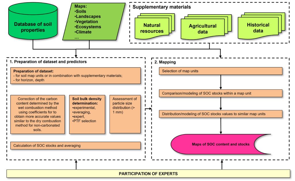
Figure 1. Flowchart of mapping based on available thematic maps
Below is the description of the main stages of SOC content and stocks mapping based on different thematic maps:
- Preparation of data and predictors includes their being divided into relatively uniform groups by the organic matter structure. The principles of dividing into groups are determined on the research purpose, the scale, characteristics, and amount of the available information, for example: by vegetation type (forest, steppe, swamp, etc.); by land use type (agricultural, residential, forest, etc.); by structure of agricultural lands (tilled field, fallow, hay field, pasture, reclaimed lands, etc.), and so on. The completeness of the available actual data on point objects, possibility of its being summarized for characterization of the classification-based and cartographic soil bodies are evaluated. Then the algorithm for the values’ recalculation by soil horizons/layers from soil profiles for the fixed targeted depths is selected, and the data is harmonized. If there is no data available for any of the soil profile depths, they are added with the mean indicators for similar objects, or with the expert knowledge-based values.
To determine the organic carbon content in soil samples, the dry combustion method based on high-temperature catalytic oxidation of the organic matter and direct accounting of the formed carbon dioxide, which ensures the maximum oxidation of the organic matter, as well as the wet combustion method based on oxidation of the organic matter with the chromic acid, are used today. Chemical methods do not lead to complete carbon oxidation of the organic compounds, so correction factors are used to correct the obtained results. The international practice widely utilizes Walkley and Black method (Walkley, Black, 1934) with the correction factor of 1.32 (Soil organic carbon…, 2018). The domestic practice more commonly employs Tyurin’s method in different modifications. B. M. Kogut and A. S. Frid (1993) proposed an averaged correction factor (K = 1.28) to recalculate the indicators obtained with the use of this method. Recent studies showed that the correction factor of 1.15 is more applicable (FAO, 2021; Shamrikova et al., 2022).
When using the high-temperature combustion method for carbonate soils, the organic carbon content is determined as a difference between the total carbon content and the carbon content of inorganic compounds.
The SOC content in soils is often converted to the humus content using the correction factor of 1.724. The correction factor was proposed in the 19th century based on data indicating that humic acid contains 58% carbon and is widely accepted for inorganic soil horizons. Due to the diversity of organic horizons, the carbon content in them varies significantly. The number of results of direct carbon determination using the dry combustion method is limited. In most cases, literature provides ignition loss data as a characteristic of the horizon’s enrichment with organic matter. For organic horizons, the correction factors may vary from 1.9 to 2.5 (Soil organic carbon…, 2018). To calculate the carbon content of forest litter, the Russian studies utilize different correction factors from 2.0 (Alekseev, Berdsi, 1994) to 2.6 (Schepaschenko et al., 2013).
For carbon stock estimation in soils, the critical calculation parameter is the soil bulk density in its natural state. In case of a lack of soil bulk density measurements, mean or median values are used, that are obtained on the available experimental data. Pedotransfer functions (PTF) are widely used to calculate the soil bulk density value based on other available soil properties. PTF are empirical and have a limited scope of application, therefore, they should be used with caution under conditions different from those for which they were obtained. The vast diversity of Russian natural and geographic conditions makes the selection of PTF a crucial stage, as it allows determining soil bulk density in a particular region with a minimum error. A comparative analysis of the five methods of soil bulk density determination showed that PTF demonstrates the best results for the mineral horizons of the European Russia forest soils, as suggested by O. V. Chestnyh and D. H. Zamolodchikov (2004) (Chernova et al., 2020). The applicability of PTF for genetically similar soil groups is also demonstrated in other studies (Pastuhov et al., 2016; Chernova et al., 2021). The organic horizon bulk density is rarely determined by an experiment, and this indicator is also characterized by a high variability, both spatial and determined by the horizon specific features. To calculate the carbon stocks in forest litter, the expert knowledge values may be used taking into account the vegetation type and age (Soil organic carbon…, 2018). To assess organic carbon stocks in peat soils of various regions, the generalized data about peat bulk density may be utilized, depending on its maturity, degree of decomposition, and ash content, for example, of peat soils in tropics (Agus et al., 2011) or Western Siberia (Inisheva et al., 2012).
Assessment of stones and gravel content, i.e. particles with a size exceeding 1 mm, is crucial for mineral soils, especially in mountain regions and soils formed on weak-weathered deposits. The researchers rarely have a sufficient number of rockiness measurements for different soils and soil horizons to calculate the mean values. In most cases, correction factors are applied for similar soil groups, which have been obtained by expert knowledge based on the summarized studies results typical for a relevant group of soil profiles (Soil organic carbon…, 2018).
The data preparation stage is completed by calculating the organic carbon stocks in soil horizons, layers or target depths, followed by calculating the mean arithmetic values for each spatial map unit.
- Mapping consists of preparing the set of predictors, determined by the objective of the study, and the available dataset, using spatial identification in GIS. Then the predictor properties are determined for each soil profile and the list of spatial mapping units is created, which are characterized by similar conditions (type/subtype/class of soil, landscape, land use, etc.). Covariates are extracted for the contours provided with a sufficient amount of fieldwork samples, the carbon content/stock values of these contours are averaged. In the case of complex soil cover, the weight coefficient can be introduced for the averaging process, which takes into account the soil composition by area ratios of the dominating, associating, and associated soils. The averaged values are assigned to all spatial mapping units that are similar in terms of soil properties, regardless of the soil profile location.
The accurate assessment of spatial uncertainty for maps constructed is challenging. Mapping errors may be caused by several reasons, including uncertainties in the boundary zones; errors in determination of the mean values for mapping units due to insufficient, subjective, or non-representative data samples; high natural value variability in complex soil cover conditions; laboratory and field measurement errors. However, the studies have examples of quantitative assessment of individual uncertainty aspects with a sufficient amount of analytical data. Kappa statistics can be used (Rossiter, 2001) to estimate the coherence between fieldwork data and final map (Pastuhov et al., 2016) or to compare two detailed soil maps compiled by two independent research groups (Samsonova, Meshalkina, 2011).
The final stage of the work is to assess and correct the results by a group of soil scientists from the study area. The examples of the organic carbon stock regional mapping according to the described approach are provided in Appendix A.
Let’s review one of the examples of the first approach. The scientist group suggested a method of obtaining the approximate regional assessment of the soil organic carbon stocks under an insufficient amount of fieldwork data samples (Chernova et al., 2016). The calculations involve the available diverse data sources, including maps, databases, government statistical databases, published results of local studies, and the carbon cycle modeling results. The method was employed in the European Russia regions: Kostroma and Kursk.
The cartographic base for the area-based calculations was obtained by overlaying the vector map layers: the corrected digital version of the RSFSR soil map (2007), the USSR vegetation map (1990) at the level of dominating vegetation type, and the Russian administrative division of 1:1 000 000-scale. We considered the following parameters during the calculations: taxonomic units of soils, particle size distribution, land use, type-age structure of forest, and peat deposit data in the regions.
The carbon stocks in autonomous natural soils were predicted using the carbon cycle nonlinear model — NAMSOM (Nonlinear Analytical Model of Soil Organic Matter) (Ryzhova, Podvezennaja, 2003) for each soil type/subtype, accounting for particle size distribution. Values from the available databases were used as a substitution for the lacking fieldwork data for both soil types and plant associations. The next step was averaging the values within the boundaries of the Environmental Zoning Map soil provinces at a scale of 1:15 000 000 (2011). The obtained averaged values were corrected, accounting for the land use types (tilled fields, hay fields, pastures; fallows; forests of different ages and non-forest woody vegetation; cut-over and burn-outs lands; swamps; roads; mixed urban and built-up lands and others).
This approach was applied for the calculation of soil organic carbon stocks in Kostroma (southern boreal forest) and Kursk (forest-steppe) regions. Reduction of carbon stocks for the historical period was approximately estimated for different regions depending on their natural, geographic, and economic conditions.
Approach II — Digital soil mapping (DSM)
The modern methods for soil properties mapping are based on the SCORPAN model, widely used in digital soil mapping recently. The SCORPAN model was suggested for the empirical quantitative description of relations between soil properties and environmental variables. The equations of SCORPAN models are presented according to McBratney et al. (2003) and Florinskij (2012).
Sс = f (s, c, o, r, p, a, n) and Sа = f (s, c, o, r, p, a, n), (1)
where Sc: soil classes; Sa: quantitative soil properties; s: soil, other properties of the soil at a point; c: climate, climatic properties of the environment at a point; o: organisms, including land cover and natural vegetation; r: topography, including terrain attributes and classes; p: parent material, including lithology; a: age, the time factor; n: space, spatial or geographic position.
Equation 1 is the result of work of many soil scientist generations, including S. A. Zaharov (1927), C. F. Shaw (1930), H. Jenny (1941), who developed the main law of the soil science proposed by V. V. Dokuchaev (Florinskij, 2012). It combines genetic and formal approaches in soil science. Digital soil mapping requires a large amount of point-based soil surveys with known spatial referencing. In case of an increase in predictor numbers and their combinations, the required amount of surveys increases. Further work on the development of an optimal sampling plan for digital soil mapping purposes led to the creation of the specialized Latin hypercube method. The method is based on selecting the sample locations depending on the probability of occurrence of dummy variables (Minasny, McBratney, 2006).
DSM includes intelligent data analysis, geostatistics, hybrid approaches and involves the completion of three consecutive stages (Fig. 2).
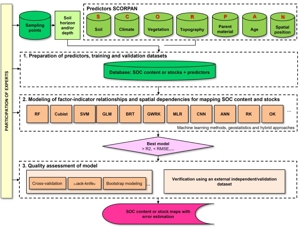
Figure 2. Flowchart of digital soil mapping of organic carbon content and stocks
Below is the description of the main stages of digital soil mapping of SOC content and stocks:
- Preparation of predictors, training, and validation datasets.
The training and validation datasets require the following information: plot identification number, geographic coordinates, soil type, soil horizonation and layer designations, range of depths, soil bulk density of horizons, SOC content and stocks, coarse soil (stones and gravel) content. In the absence of soil bulk density data, researchers employ simulations of the pedotransfer functions; results are included in both training and validation datasets.
The spatial predictors used for modeling the SOC content and stocks describe soil formation factors and indicator variables. As a topographic representation of the surface, we used a digital terrain model to calculate relief morphometric parameter maps. A morphometric parameter is a numerical characteristic of the relief determined at a point on the surface. These parameters represent multiple features of the surface topography: elevation, slope, aspect, etc. (Sharyj, 2006). The specified morphometric parameters are among the main aspects of the terrain effect on functionality of the ecosystem along with terrain dissection, geometry and slope thermal regime. P. Sharyj (2006) and I. Florinskij (2016) systematized the main aspects of the terrain effect which included surface runoff, terrain dissection, geometry, slope thermal regime, and vertical zonation. According to the system of the basic morphometric parameters, the surface runoff is described by slope orientation and steepness; horizontal, vertical, difference, and accumulation curvature; catchment area and dispersive area. The morphometric variables that determine terrain dissection are horizontal and vertical excessive curvature; ring curvature; rotor. The morphometric variables that describe the terrain geometry are unsphericity curvature; minimum, maximum, and mean curvature; Gaussian curvature. Slope thermal regime is determined by their illumination, vertical zonation is determined by the Earth’s surface altitude.
Preparation of predictors characterizing vegetation involves the use of multispectral images as a basis for the computation of various indicators. It includes vegetation indices and reflection in the blue, red, green, and near-infrared spectrum. Environmental variables that characterize climate and parent materials (Appendix B) are utilized as the predictors for the SOC content and stocks mapping. SAGA GIS, QGIS, ArcGIS, and a cloud platform Google Earth Engine (GEE) are most frequently utilized for predictors development. The SOC content and stocks are commonly simulated in R, QGIS, ArcGIS, SAGA GIS, and other software.
- Modeling factor-indicator relationships and spatial dependencies is performed using machine learning (ML) methods — decision trees (DT, RF, BaRT, BRT, CART), kriging (OK, RK, GWRK), neural networks (ANN, CNN), linear regressions (GLM, MLR), and others. The literature review showed the predominant use of the following ML methods: random forest (RF, utilized in 24% of the observed studies), regression kriging (RK, 11%), and support vector machine (SVM, 7%) (Appendix A).
In some studies, the authors use multiple machine learning methods to model SOC stocks — GWRK and RK (Kumar et al., 2012); BART, RF, XGBoost (Chinilin, Savin, 2018); RF, Cubist, RK (Kaya et al., 2022). Researchers pay attention to the insufficiency of using just one simulation method and the feasibility of testing different models for a certain mapping territory. The “Methods” column in Appendix A includes the list of all used methods. The methods in bold demonstrated the best results of the SOC content or stocks simulation. The factor-indicator relations are simulated in these methods based on the learning dataset, where the carbon content/stocks and predictor values are known at certain points. Simulated relations then are used for “recognition” of the rest of the mapping territory, with the available predictors, but unknown amount of carbon content/stocks. The machine learning methods may be supplemented by studying the spatial dependencies and interpolation methods applications (ex. simple kriging method). The map obtained in such manner has to be verified. Many studies use jackknife, cross-validation, or bootstrap methods to assess model quality. The most advantageous verification approach is an additional (independent) probability sampling.
Random forest is a machine learning algorithm that involves the use of a set of decision trees (Breiman, 2001). The algorithm of the decision tree creation or recursive decomposition suggests the choice of a variable and a cut-off point resulting in the best classification results. Then compliance with the stopping criteria is verified for each resulting path. The stopping criterion is typically a certain depth of the tree growth or the minimum number of surveys for which further classification by the leaf is impossible. According to the algorithm, sample subsets are formed from the main sample set with a replacement (bootstrap). An individual model of the decision tree is compiled for each sample subset. The method was called the random forest, because it summarizes a large set of trees obtained based on random samples. The final model is a weighted mean of all compiled decision trees.
The use of this method includes the following advantages: high forecasting capacity; absence of re-training; low intercorrelation of individual trees, since the variety of the forests increases due to the use of a limited number of prediction variables; low displacement and dispersion due to the averaging over numerous trees. The predictors in this method can be both qualitative and quantitative, and there is no distribution normality requirement for the quantitative indicators, as the method is classified as non-parametric. One of the main disadvantages of the method is the internal complexity of the resulted forest of models, which complicates interpretation of interdependencies between dependent variables and predictive variables, as it is impossible to study the structure of all trees in the forest.
Regression kriging is a hybrid method that combines simple or multiple linear regression with the kriging of forecast residuals. The principle of the method is finding a relation between the predictors and the carbon content/stocks, using regression or machine learning methods, in which case the term “regression kriging” is used in a wider sense. Then the residuals are verified for the presence of spatial dependencies. The limitations of the method include a training dataset of at least 100–150 sample points; the fulfillment of the stationarity condition for residuals — transitivity of the variogram; and the normal distribution of residuals.
Support vector machine is also classified as a non-parametric machine learning method. The method is to input the initial vectors to a very high-dimension feature space and to find а separating hyperplane with a maximum gap in it (Vapnik, 1998). Two parallel hyperplanes are plotted on both sides of a hyperplane separating the classes. The algorithm works on the assumption that the bigger difference or distance between the parallel hyperplanes are, the lesser a mean error of the classifier is.
The advantages of the support vector machine are its efficiency in larger-size spaces and in cases when the number of attributes exceeds the number of surveys (Pedregosa et al., 2011). A subset of learning points is used in the decision-making function, which is why this method is efficient in terms of the use of computer memory. The method is characterized by its flexibility: different core functions can be set for the decision-making function, and the user can also set their own support vectors.
- Model evaluation and uncertainty analysis are performed with the use of an independent validation dataset or the model stability can be verified with the use of jackknife, cross-validation, and bootstrap simulation methods. To estimate the accuracy of the maps, different indicators are used, such as the root mean squared error or the mean absolute percentage error.
The use of an independent dataset for the model test. To test the map model, it is recommended to use the specialized additional (independent) probability sample dataset. Ideally, this sampled dataset is created individually as a result of independent fieldwork in the study area. Here, “probability” refers to the fact that the dataset is representative for the surveyed territory, i.e. probability of objects (points) entering the sampled dataset is equal to the probability of their representation on the territory depending on the level of its non-uniformity. For example, if a territory includes different soil types and subtypes, they should be represented in the sampled dataset with the same probability as on the territory.
In case of absence of independent field data, the sampling points is divided into two datasets: training and validation. The training dataset is used for plotting the models. The validation dataset is generally 10 to 30% (20% on average) of the total dataset, depending on the number of points. It should be tested for representativity as related to the total dataset. It is critical that the independent or validation dataset is created once and used for testing the model upon completion of simulation.
Model stability test. Jackknife, cross-validation, and bootstrap simulation are classified as the methods for creating a sufficiently large number of subsamples based on a single population sample. Subsamples can be used for different purposes both during simulation and for modeling tests. In any case, subsamples are dependent on the population sample. If the initial population sample contains distortions, the subsamples obtained with the use of the above-mentioned methods would have the same distortions. When using the methods listed, only the model stability is tested, without verifying its compliance with the studied territory.
Jackknife method (element-by-element cross-validation) involves systematic recalculation of the required statistics (mean, median, correlation or regression factors, etc.) by deleting surveys from the sampled dataset randomly one by one. Some of the surveys can be “discarded”, but generally the procedure is being continued until all survey points are captured. This way, an unbiased estimate and error of the statistics can be obtained.
The jackknife procedure has a less generalized nature as compared to the bootstrap simulation. However, the jackknife is simpler to use for complicated sampling schemes, such as multi-stage sampling with different weights. The jackknife and the bootstrap simulation often yield the same results. At the same time, the bootstrap simulation can have slightly different results for repeatability with the same data, while the jackknife has the same result every time (provided that the subsets are selected from the same sampled dataset). The jackknife is often used due to the simplicity of the procedure and the possibility of visual representation of the results in the form of a graph of observed and predicted values.
Cross-validation method (cross-check, running control, maximum impartiality method) involves random division of the subset of surveys into training and validation datasets. Based on the training dataset, the model is adjusted, and based on the second dataset, the model is tested. This process is repeated multiple from 10 to 100 or up to 1000 times. The forecast accuracy measure is considered to be a mean estimation obtained based on the results of each value of the validation dataset.
Bootstrap simulation is a statistical method of the random value distribution estimation, under which subsamples with a replacement (i. e. subsamples are returned to the initial sample every time) are taken from the initial sample for a sufficient number of times. Generally, the subsamples constituting 99%, 95% or 90% of the initial sample are taken (Meshalkina et al., 2010). As a result of such procedure, an error or a confidence interval are obtained for the general set parameters — mean, median, correlation or regression factors. The bootstrap simulation is used for creation and verification of hypotheses in case of a small initially sampled dataset.
Indicators used for verification of accuracy of the qualitative soil properties maps. All indicators for the verification of digital maps (Table 1) of the qualitative soil properties, including the carbon stocks and/or content, are based on the analysis of residuals or mis-ties obtained as the difference e(si) of the values predicted by the map model (si) and the observed values Z(si) at points (si) used for verification:
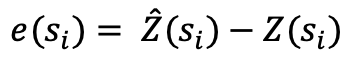
Table 1. Basic indicators used to estimate accuracy of qualitative soil properties maps
| Mean absolute error, MAE | 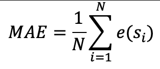 |
|
| Mean squared error, MSE | 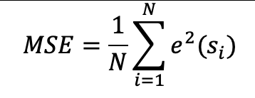 |
|
| Root mean squared error, RMSE | 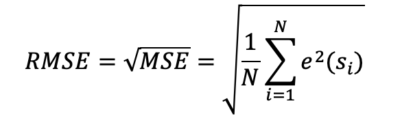 |
|
| Mean absolute percentage error, MAPE | 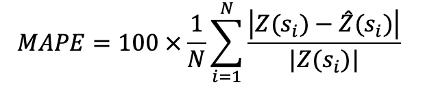 |
|
| Amount of variance explained, AVE | 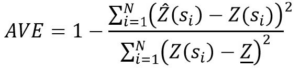 |
|
| Mean squared deviation ratio, MSDR | 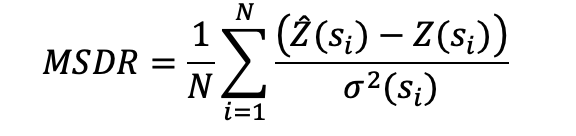 |
Legend: e(si) is the difference between predicted and observed values; ![]() is the predicted value; Z(si) is the observed value; N is the number of sampling points in the analyzed/validation dataset; is the dispersion; Z is the average value of soil property in the analyzed dataset
is the predicted value; Z(si) is the observed value; N is the number of sampling points in the analyzed/validation dataset; is the dispersion; Z is the average value of soil property in the analyzed dataset
Mean absolute error (MAE) and mean squared error (MSE) demonstrate the mapping accuracy and reflect a mean mis-tie correction. They are used when it is required to detect large errors and choose the model providing fewer large forecasting errors. When using one of these estimations, it can be useful to analyze which objects contribute the most to the total error: it is not unlikely that an error was made in these objects during the calculation of predictors and SOC content/stocks. Root mean squared error (RMSE) is used more often, as it has the same unit of measurement as the initial data. This indicator is highly dependent on the presence of large mis-tie values, so generally not mean, but the median value of MSE is calculated, and then the root is extracted from it. Mean absolute percentage error (MAPE) can be measured in fractions or percent. For example, MAPE = 6% means that the error was 6% of actual values. The main problem of this error is instability.
Amount of variance explained (R2) or “model efficiency”, shows a percentage of dispersion explained by the model from the total dispersion of the predicted variable. Technically, this quality measure is a normalized mean squared error. If it is close to one, the model explains data well, if it is close to zero — the forecast quality is comparable to the prediction by a mean value only. Mean squared deviation ratio (MSDR) shows how well the model predicts simulation uncertainty. If kriging was applied to residuals, the prediction uncertainty would comply with the kriging error.
Analysis of used predictors. Literature analysis showed that the terrain-based covariates were the most frequently used environmental variables, followed by the variables representing vegetation and climate (Fig. 3, Appendix A). Taxonomic units of soils significantly improved the mapping accuracy, but this data was utilized in only 5.6% of the research studies.
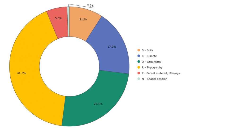
Figure 3. The percentage ratio of predictors examined in the literature review within the SCORPAN model (Appendix B)
The following predictors were the most informative in the digital mapping of SOC content and stocks: taxonomic units of soils, annual precipitation, NDVI, elevation, slope, topographic wetness index (Appendix B, Fig. 4, 5).
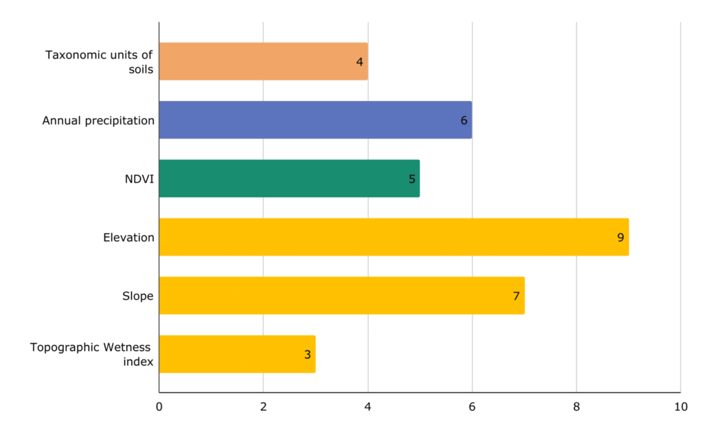
Figure 4. The most informative predictors based on the literature review (Appendix B)
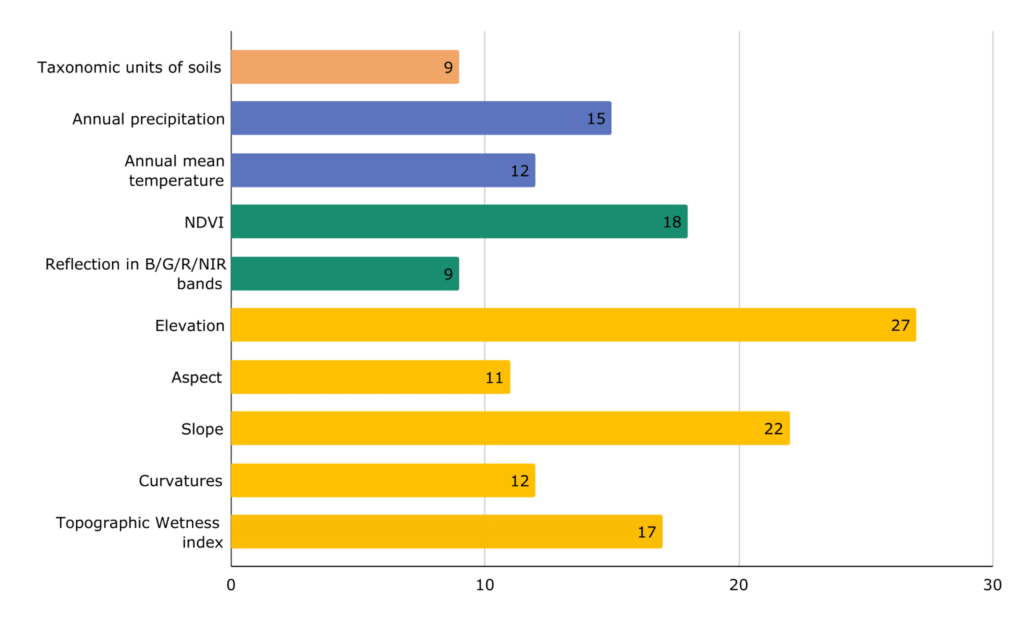
Figure 5. The 10 most commonly used predictors for mapping of SOC content and stocks in soils are based on the literature review (Appendix B)
In this study, we organized the review based on the Earth’s biomes, relying on D. Olson’s map (Olson et al., 2001) (Fig. 6). For literature capturing multiple biomes simultaneously, we considered all biomes located within the boundaries of the study area. Most of the research works were conducted in temperate broadleaf and mixed forests (4), then Mediterranean forests, woodlands, and scrub (12); deserts and xeric shrublands (13); temperate grasslands, savannas, shrublands (8) (Fig. 6). The present study is not comprehensive, the represented distribution on the graph may change when new publications appear.
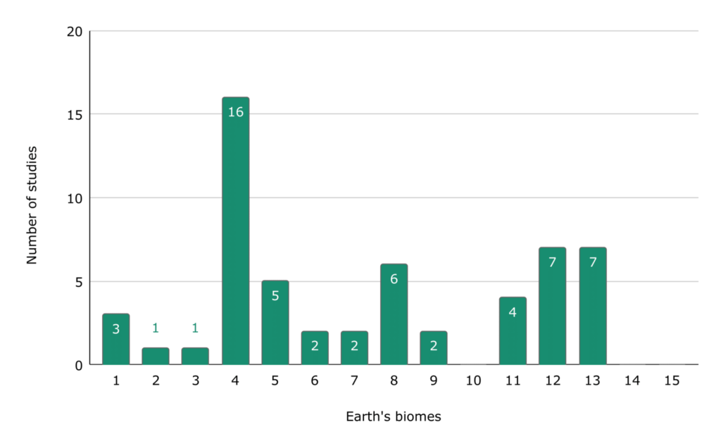
Figure 6. Distribution of the SOC content/stock mapping studies organized by Earth’s biomes (Olson et al., 2001) at the regional and local scales: 1 — tropical and subtropical moist broadleaf forests; 2 — tropical and subtropical dry broadleaf forests; 3 — tropical and subtropical coniferous forests; 4 — temperate broadleaf and mixed forests; 5 — temperate coniferous forests; 6 — boreal forests/taiga; 7 — tropical and subtropical grasslands, savannas, and shrublands; 8 — temperate grasslands, savannas, shrublands; 9 — flooded grasslands and savannas; 10 — mountain grasslands and shrublands; 11 — tundra; 12 — Mediterranean forests, woodlands, scrub; 13 — deserts and xeric shrublands; 14 — mangroves; 15 — polar deserts
Geographic distribution. The review of recent publications shows that digital soil mapping at the regional and local level scales is the most trending approach for SOC content and stock mapping. These studies are conducted on every continent, excluding Antarctica (Fig. 7). In Russia, regional and local studies have been done in Voronezh (Chinilin, Savin, 2018), Bryansk (Gavrilyuk et al., 2021) and Novosibirsk (Gopp, 2022) regions, Krasnoyarsk krai (Sharyj et al., 2018), the Republic of Bashkortostan (Suleymanov et al., 2021) and the Republic of Karelia (Narykova, Plotnikova, 2022). An accurate quantitative estimation of SOC stocks in soil is problematic, mostly due to the sparsity of sampling data, especially at large soil depths. It leads to considerable uncertainty and discrepancies in results among different authors by 2-3 times (Piao et al., 2009; Sharyj et al., 2018).
The first publications about DSM date back to the 1980s. In 2003, A. McBratney et al. issued the article “On Digital Soil Mapping”, where they introduced the main principles of the approach. Australia, Netherlands, the USA, and France became the main development centers of this approach (Lagacherie et al., 2007; Hartemink et al., 2008).
In November 2008, the global project GlobalSoilMap.net (GlobalSoilMap.net…, 2008) was launched to create a digital soil map of the world, based on chorograms of soil properties. Methodological justification of the project could be found in the journal Science (Sanchez et al., 2009). The following soil properties were declared as subject to mapping: carbon and gravel content, particle size distribution, soil bulk density, and available water capacity. These properties had to be estimated at six depths (in cm): 0–5, 5–15, 15–30, 30–60, 60–100, and 100–200 with an indication of the mean values and the confidence intervals. The authors planned to map 80% of the global land surface with a spatial resolution of 90 m. Currently, the project has been implemented only for African countries.
SoilGrids project (SoilGrids — Global Gridded Soil Information) is a system of digital soil mapping that employs modern machine learning methods to visualize the spatial distribution of the following soil properties at the global scale: organic carbon content, total nitrogen, particle size distribution (sand, clay, silt), water extraction pH, cation exchange capacity, and soil bulk density. SoilGrids 2.0 mapping models are based on more than 240 000 soil samples obtained from the International Soil Reference Information Center, ISRIC (WoSIS database), and the global environmental covariates (more than 400) that represent vegetation, terrain, climate, geology, and hydrology (Poggio et al., 2021). The global maps of soil properties with the spatial resolution of 250 m are represented in this system following the specifications of GlobalSoilMap IUSS working group for six standard depth intervals (0–5, 5–15, 15–30, 30–60, 60–100 and 100–200 cm). The map represents the soil organic carbon stocks for the 0–30 cm soil layer.
GLOSIS (Global Soil Information System) platform summarizes soil data collected by national institutions (URL: https://goo.su/V3Jw). The platform features the global map of the SOC stocks for the layer of 0–30 cm called GSOCmap v.1.5.0 (FAO and ITP …, 2018) with 30 arc-second (approximately 1 km) resolution. Part of the map related to the Russian is modeled on the corrected digital version of the RSFSR soil map at a scale of 1:2 500 000 and Information System Soil-Geographic Database of Russia (ISSGDB) with fieldwork data from the 1960s–1980s (Chernova et al., 2021).
Multiple studies of SOC content and stocks mapping have been performed in European countries (CEF Telecom project, 2018): Netherlands (Wadoux et al., 2022); Denmark (Adhikari et al., 2014); Scotland, Great Britain (Poggio, Gimona, 2014); Bavaria, Germany (Wiesmeier et al., 2014); Belgium (Meersmans et al., 2008); France (Arrouays et al., 2001; Chen et al., 2018; Martin et al., 2011; Meersmans et al., 2012; Mulder et al., 2016); Switzerland (Nussbaum et al., 2014; Zhou et al., 2021); Hungary (Szatmari et al., 2021); Italy (Fantappie et al., 2011; Francaviglia et al., 2014); Ukraine (Viatkin et al., 2018). Mapping of carbon stocks in Asian countries is primarily developed in China (Wiesmeier et al., 2011; Zhou et al., 2019; Wang et al., 2021; Gu et al., 2022; Zhu et al., 2022; Guo et al., 2015) and Iran (Taghizadeh-Mehrjardi et al., 2016; Hateffard et al., 2019; Fathizad et al., 2022; Kaya et al., 2022). There are several studies in India (Lo Seen et al., 2010) and Tibet (Yang et al., 2008).
Examples of studies at the regional scale include mapping in different regions of the world, including the US: Pennsylvania (Kumar et al., 2012), Wisconsin (Adhikari et al., 2019), Florida (Kim, Grunwald, 2016; Keskin et al., 2019), Indiana (Mishra et al., 2009); in South America: Chili (Rojas et al., 2018; Padarian et al., 2017), Brazil (Bonfatti et al., 2016; Gomes et al., 2019) and Columbia (Rainford et al., 2021); in Africa: South Africa (Venter et al., 2021) and Mozambique (Cambule et al., 2014); Australia (Gray, Bishop, 2016; Padarian et al., 2019; Somarathna et al., 2016; Wang et al., 2018).
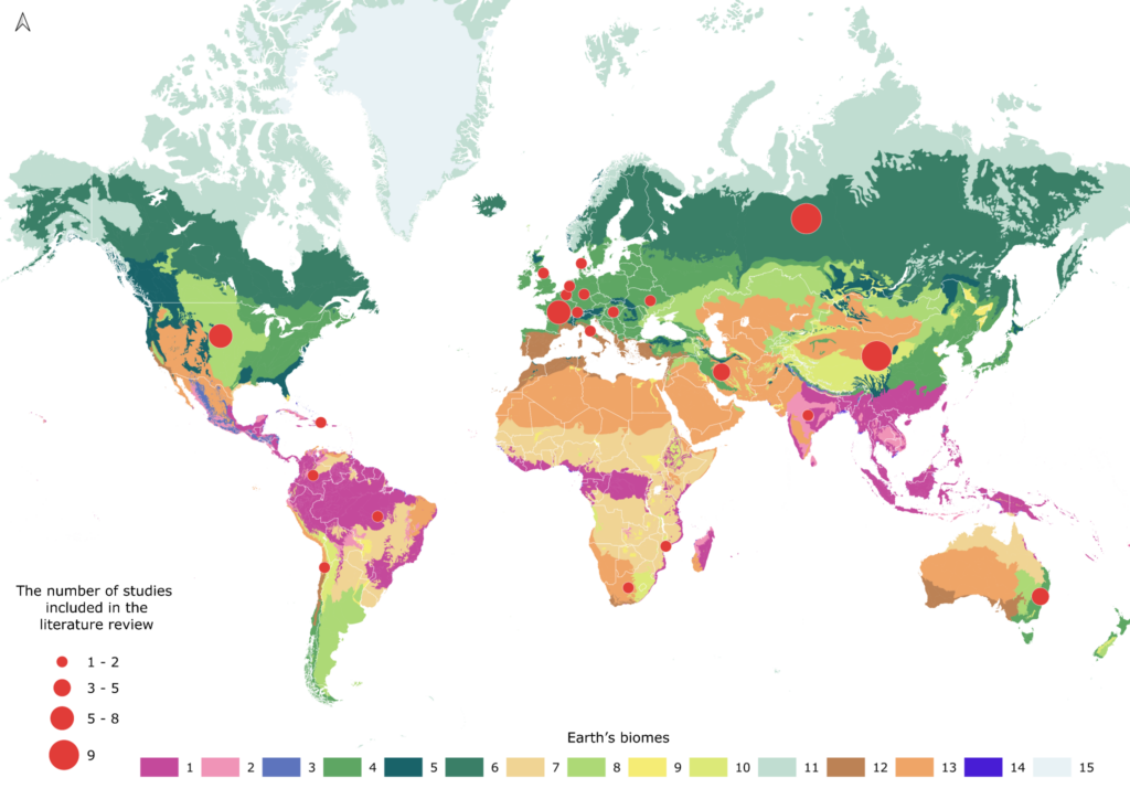
Figure 7. Geography of the reviewed studies of soil organic carbon content/stocks mapping at the regional and local scales (Olson et al., 2001): 1 — tropical and subtropical moist broadleaf forests; 2 — tropical and subtropical dry broadleaf forests; 3 — tropical and subtropical coniferous forests; 4 — temperate broadleaf and mixed forests; 5 — temperate coniferous forests; 6 — boreal forests/taiga; 7 — tropical and subtropical grasslands, savannas, and shrublands; 8 — temperate grasslands, savannas, shrublands; 9 — flooded grasslands and savannas; 10 — mountain grasslands and shrublands; 11 — tundra; 12 — Mediterranean forests, woodlands, Scrub; 13 — deserts and xeric shrublands; 14 — mangroves; 15 — polar deserts
CONCLUSION
As part of the analysis of modern methodological approaches for soil organic carbon content and stock mapping, we identified and discussed two approaches: (1) based on the existing thematic maps and archive data; and (2) digital soil mapping combining spatial data analysis. It is reasonable to use both approaches for mapping organic carbon content and stocks in Russia. For each approach, the authors formulated the conditions of application and the necessary steps. Mapping based on thematic maps and archive data includes two stages: preparation of data and predictors utilizing GIS; mapping of SOC content and stocks by the land use type and taxonomic units of soils. Verification is based on expert assessment.
Digital mapping is performed in three stages: preparation of two independent datasets (training and validation) and environmental variables (predictors); modeling of the factor-indicator relationships and spatial dependencies, followed by a model quality assessment. The factor-indicator relationships are employed by machine learning methods, geostatistics, and hybrid approaches (RF, BRT, SVM, GLM, MLR, CART, ANN, CNN, RK, OK and others). Various kriging methods are used to determine spatial dependencies of residuals. The quality assessment of the model, measuring the level of agreement between the map model and actual data, is verified using an independent validation dataset referred to as the “independent probability sample” in digital soil mapping. Simulation quality in this case can be assessed with the use of an interpolation error map. The model quality assessment is performed with the use of jackknife, cross-validation, and bootstrap methods, which represents how the model describes the training sample. Different criteria are used to estimate the accuracy of the quantitative properties map, such as MAE, MSE, RMSE, MAPE, etc.
To map the SOC content and stocks at the local and regional level scales, authors are required to use a training sample and a set of spatial predictors that represent the soil formation factors based on the SCORPAN model.
Environmental covariates represent the following data: vegetation (vegetation type, land use type); climate (annual mean temperature, annual precipitation); topography (relief morphometric parameters); parent materials and soil (genetic types of parent materials, taxonomic units of soils, chemical and physical soil properties, permafrost distribution); anthropogenic effect (land use type, cut-overs, burn-outs). In addition to the data obtained from the archive sources, digital soil mapping uses remote sensing data to calculate different indicators, including at least 200 indicators for vegetation, 40 for terrain, and 10 for soil parent materials.
Therefore, the performed literature review allowed us to determine specific features of the main methodological approaches used for the soil organic carbon content and stock mapping nearly in all global continents and different Earth’s biomes. The progress achieved in the digital soil mapping is still insufficient for Russian territory.
The number of studies on this topic is low, so the comparative assessment of the soil properties heterogeneity mapping results based on available multi- and hyperspectral images, the digital models of altitudes and radar images in different terrestrial ecoregions are underserved in the literature. We hope studies involving the use of DSM will be continued, and advanced methods that would allow to process of remote sensing data, identify, and estimate the variability of soils and soil properties would be developed.
FUNDING
The research was performed as part of the most important innovative project of national importance “Development of a system for ground-based and remote monitoring of carbon pools and greenhouse gas fluxes in the territory of the Russian Federation, ensuring the creation of recording data systems on the fluxes of climate-active substances and the carbon budget in forests and other terrestrial ecological systems” (Reg. No 123030300031-6).
REFERENCES
Adhikari K., Hartemink A. E., Minasny B., Kheir R. B., Greve M. B., Greve M. H., Digital mapping of soil organic carbon contents and stocks in Denmark, PLoS ONE, 2014, Vol. 9, No 8, Article: e105519.
Adhikari K., Owens P., Libohova Z., Miller D., Wills S., Nemecek J., Assessing soil organic carbon stock of Wisconsin, USA and its fate under future land use and climate change, Science of The Total Environment, 2019, Vol. 667, pp. 833–845.
Agus F., Hairiah K., Mulyani A., Measuring carbon stock in peat soils: practical guidelines. Bogor, Indonesia: World Agroforestry Centre (ICRAF) Southeast Asia Regional Program, Indonesian Centre for Agricultural Land Resources Research and Development, 2011, 60 p.
Alekseev V. A., Berdsi R. A., Uglerod v ekosistemah lesov i bolot Rossii (Carbon storage in forests and peatlands of Russia), Krasnoyarsk: VC SO RAN, 1994, 226 p.
Arrouays D., Deslais W., Badeau V., The carbon content of topsoil and its geographical distribution in France, Soil Use and Management, 2001, Vol. 17, Issue 1, pp. 7–11.
Bonfatti B. R., Hartemink A. E., Giasson E., Tornquist C. G., Adhikari K., Digital mapping of soil carbon in a viticultural region of Southern Brazil, Geoderma, 2016, Vol. 261, pp. 204–221.
Breiman L. Random Forests, Machine Learning, 2001, Vol. 45, No 1, pp. 5–32.
Cambule A. H., Rossiter D. G., Stoorvogel J. J., Smaling E. M. A., Soil organic carbon stocks in the Limpopo National Park, Mozambique: amount, spatial distribution and uncertainty, Geoderma, 2014, Vol. 213, pp. 46–56.
CEF Telecom project 2018-EU-IA-0095: “Geo-harmonizer: EU-wide automated mapping system for harmonization of Open Data based on FOSS4G and Machine”, available at: URL: https://ecodatacube.eu/ (February 25, 2023).
Chen S., Martin M. P., Saby N. P. A., Walter C., Angers D. A., Arrouays D., Fine resolution map of top- and subsoil carbon sequestration potential in France, Science of The Total Environment, 2018, Vol. 630, pp. 389–400.
Chernova O. V., Golozubov O. M, Aljabina I. O., Schepaschenko D. G., Kompleksnyj podhod k kartograficheskoj ocenke zapasov organicheskogo ugleroda v pochvah Rossii (Integrated approach to spatial assessment of soil organic carbon in Russian Federation), Eurasian Soil Science, 2021, No 3, pp. 273–286.
Chernova O. V., Ryzhova I. M., Podvezennaja M. A., Ocenka zapasov organicheskogo ugleroda lesnyh pochv v regional’nom masshtabe (Assessment of organic carbon stocks in forest soils on a regional scale), Eurasian Soil Science, 2020, No 3, pp. 340–350.
Chernova O. V., Ryzhova I. M., Podvezennaja M. A., Opyt regional’noj ocenki izmenenij zapasov ugleroda v pochvah juzhnoj tajgi i lesostepi za istoricheskij period (An experience in regional estimates of changes in soil carbon pools of the southern taiga and forest-steppe during the historical period), Eurasian Soil Science, 2016, No 8, pp. 1013–1028.
Chestnyh O. V., Zamolodchikov D. G., Zavisimost’ plotnosti pochvennyh gorizontov ot glubiny ih zaleganija i soderzhanija gumusa (Bulk density of soil horizons as dependent on their humus conten), Eurasian Soil Science, 2004, No 8, pp. 937–944.
Chinilin A. V., Savin I. Ju., Krupnomasshtabnoe cifrovoe kartografirovanie soderzhanija organicheskogo ugleroda pochv s pomoshh’ju metodov mashinnogo obuchenija (The large scale digital mapping of soil organic carbon using machine learning algorithms), Bjulleten’ Pochvennogo instituta im. V. V. Dokuchaeva, 2018, Vol. 91, pp. 46–62.
Dobrovol’skij G. V., Urusevskaya I. S., Alyabina I. O., Karta pochvenno-geograficheskogo rajonirovaniya (Map of soil-geographical zoning), In: Nacional’nyj atlas pochv Rossijskoj Federacii (National Soil Atlas of Russia), Moscow, 2011, pp. 196–201.
Duarte E., Zagal E., Barrera J., Dube F., Casco F., Hernandez A., Digital mapping of soil organic carbon stocks in the forest lands of Dominican Republic, European journal of remote sensing, 2022, Vol. 55, No 1, pp. 213–231.
Ellili Y., Walter Ch., Michot D., Pichelin P., Lemercier B., Mapping soil organic carbon stock change by soil monitoring and digital soil mapping at the landscape scale, Geoderma, 2019, Vol. 351, pp. 1–8.
Fantappie M., L’Abate G., Costantini E., The influence of climate change on the soil organic carbon content in Italy from 1961 to 2008, Geomorphology, 2011, Vol. 135, Issues 3–4, pp. 343–352.
FAO and ITPS, Global Soil Organic Carbon Map (GSOCmap) Technical Report, 2018. Rome. 162 p.
FAO, Standartnaja rabochaja metodika dlja organicheskogo ugleroda pochvy. Spektrofotometricheskii metod Tjurina (Standard operating procedure for soil organic carbon. The Tyurin spectrophotometric method), 2021, 26 p., available at: URL: https://goo.su/cvVhzWh (February 15, 2023).
Fathizad H., Taghizadeh-Mehrjardi R., Hakimzadeh Ardakani M. A., Zeraatpisheh M. Heung B., Scholten T., Spatiotemporal Assessment of Soil Organic Carbon Change Using Machine-Learning in Arid Regions, Agronomy, 2022, Vol. 12, Issue 3, No 628.
Florinskij I. V., Gipoteza Dokuchaeva kak osnova cifrovogo prognoznogo pochvennogo kartografirovanija (k 125-letiju publikacii) (The Dokuchaev hypothesis as a basis for predictive digital soil mapping (on the 125th anniversary of its publication)), Eurasian Soil Science, 2012, No 4, pp. 500–506.
Florinskij I. V., Illjustrirovannoe vvedenie v geomorfometriju (An illustrated introduction to geomorphometry), Jelektronnoe nauchnoe izdanie Al’manah Prostranstvo i Vremja, 2016, Vol. 11, No 1, pp. 1–20.
Francaviglia R., Renzi G., Rivieccio R., Marchetti A., Piccini C., Spatial analysis and prediction of soil organic carbon in Friuli Venezia Giulia region (Northern Italy), Geoinformatic and Geostatistic: An Overview, 2014, Vol. 2, Issue 3, pp. 1–8.
Gavrilyuk E. A., Kuznecova A. I., Gornov A. V., Geoprostranstvennoe modelirovanie soderzhaniya i zapasov azota i ugleroda v lesnoj podstilke na osnove raznosezonnyh sputnikovyh izobrazhenij Sentinel (Geospatial Modeling of Nitrogen and Carbon Content and Stock in the Forest Soil Organic Horizon Based on Sentinel-2 Multi-Seasonal Satellite Imagery), Eurasian Soil Science, 2021, Vol. 54, No 2, pp. 168–182.
GlobalSoilMap.net, 2008, available at: URL: https://www.isric.org/projects/globalsoilmapnet (Februaty 03, 2023).
Gomes L., Faria R., de Souza E., Veloso G., Schaefer C., Fernandes Filho E., Modelling and mapping soil organic carbon stocks in Brazil, Geoderma, 2019, Vol. 340, pp. 337–350.
Google Earth Engine, 2017, available at: URL: https://earthengine.google.com/ (February 03, 2023).
Gopp N. V., Uglerod v pochvah Kuznecko-Salairskoj geomorfologicheskoj provincii: baza dannyh, cifrovoe kartografirovanie, geoprostranstvennyj analiz (Carbon in the soils of the Kuznetsk-Salair geomorphological province: database, digital mapping, geospatial analysis), Sbornik nauchnyh trudov Mezhdunarodnoj nauchnoj konferencii “Evolyuciya pochv i razvitie nauchnyh predstavlenij v pochvovedenii”, posvyashchennoj 90-letiyu so dnya rozhdeniya L. M. Burlakovoj (Sourcebook of the International scientific conference dedicated to the 90th anniversary of the birth of L. M. Burlakova), Barnaul, 2022, pp. 55–58.
Gorelick N., Hancher M., Dixon M., Ilyushchenko S., Thau D., Moore R., Google Earth Engine: Planetary-scale geospatial analysis for everyone, Remote Sensing of Environment, 2017, Vol. 202, pp. 18–27.
Gray J. M., Bishop T. F. A., Change in soil organic carbon stocks under 12 climate change projections over New South Wales, Australia, Soil Science Society of America Journal, 2016, Vol. 80, pp. 1296–1307.
Gu J., Bol R., Sun Y., Zhang H., Soil carbon quantity and form are controlled predominantly by mean annual temperature along 4000 km North-South transect of Eastern China, Catena, 2022, Vol. 217. Article: 106498.
Guo P.-T., Li M.-F., Luo W., Tang Q.-F., Liu Z.-W., Lin Z.-M., Digital mapping of soil organic matter for rubber plantation at regional scale: An application of random forest plus residuals kriging approach, Geoderma, 2015, Vol. 237–238, pp. 49–59.
Hartemink A., McBratney A. B., Mendonca L., Digital soil mapping with limited data. Montpellier: Springer-Verlag, 2008, pp. 3–181.
Hateffard F., Dolati P., Heidari A., Zolfaghari A., Assessing the performance of decision tree and neural network models in mapping soil properties, Journal of Mountain Science, 2019, Vol. 16, Issue 8, pp. 1833–1847.
Hugelius G., Strauss J., Zubrzycki S., Harden J. W., Schuur E. A. G., Ping C.-L., Schirrmeister L., Grosse G., Michaelson G. J., Koven C. D., O’Donnell J. A., Elberling B., Mishra U., Camill P., Yu Z., Palmtag J., Kuhry P., Estimated stocks of circumpolar permafrost carbon with quantified uncertainty ranges and identified data gaps, Biogeoscience, 2014, Vol. 11, pp. 6573–6593.
Inisheva L. I., Sergeeva M. A., Smirnova O. N., Deponirovanie i emissiya ugleroda bolotami Zapadnoj Sibiri (Deposition and emission of carbon by Western Siberian Mires), Nauchnyj dialog, 2012, No 7, pp. 61–74.
Jenny H., Factors of Soil Formation. A System of Quantitative Pedology, New York: McGraw Hill, 1941, 281 p.
Jiang J., Zhu A.X., Qin C.Z., Zhu T., Liu J., Du F., Liu J., Zhang Y., An CyberSoLIM: A cyber platform for digital soil mapping, Geoderma, 2016, Vol. 263, pp. 234–243.
Karta rastitel’nosti SSSR, Masshtab 1 : 4 000 000 (Vegetation map of the USSR, Scale 1:4 000 000), Moscow: GUGK, 1990.
Kaya F., Keshavarzi A., Francaviglia R., Kaplan G., Basayigit L., Dedeoglu M., Assessing Machine Learning-Based Prediction under Different Agricultural Practices for Digital Mapping of Soil Organic Carbon and Available Phosphorus, Agriculture, 2022, Vol. 12, Issue 7, Article: 1062.
Keskin H., Grunwald S., Harris W., Digital mapping of soil carbon fractions with machine learning, Geoderma, 2019, Vol. 339, pp. 40–58.
Kim J., Grunwald S., Assessment of carbon stocks in the topsoil using Random Forest and remote sensing images, Journal of Environmental Quality, 2016, Vol. 45, pp. 1910–1918.
Kogut B. M., Frid A. S., Sravnitel’naya ocenka metodov opredeleniya soderzhaniya gumusa v pochvah (Comparative evaluation of methods for determining humus content in soils), Eurasian Soil Science, 1993, No 9, pp. 119–123.
Kumar S., Lal R., Liu D., A geographically weighted regression kriging approach for mapping soil organic carbon stock, Geoderma, 2012, Vol. 189, pp. 627–634.
Lagacherie P., McBratney A. B., Voltz M., Digital Soil Mapping. An Introductory Perspective, Developments in Soil Science, 2007, Vol. 31, pp. 3–22.
Lo Seen D., Ramesh B. R., Nair K. M., Martin M., Arrouays D., Bourgeon G., Soil carbon stocks, deforestation and landcover changes in the Western Ghats biodiversity hotspot (India), Global Change Biology, 2010, Vol. 16, Issue 6, pp. 1777–1792.
Martin M., Wattenbach M., Smith P., Meersmans J., Jolivet C., Boulonne L., Arrouays D., Spatial distribution of soil organic carbon stocks in France, Biogeosciences, 2011, Vol. 8, Issue 5, pp. 1053–1065.
McBratney A. B., Mendoca Santos M. L., Minasny B., On digital soil mapping, Geoderma, 2003, Vol. 117, Issues 1–2, pp. 3–52.
Meersmans J., De Ridder F., Canters F., De Baets S., Van Molle M., A multiple regression approach to assess the spatial distribution of Soil Organic Carbon (SOC) at the regional scale (Flanders, Belgium), Geoderma, 2008, Vol. 143, pp. 1–13.
Meersmans J., Martin M., Lacarce E., De Baets S., Jolivet C., Boulonne L., Lehmann S., Saby N., Bispo A., Arrouays D., A high resolution map of French soil organic carbon, Agronomy for Sustainable Development, 2012, Vol. 32, No 4, pp. 841–851.
Meshalkina Yu. L., Vasenev I. I., Kuzyakova I. F., Romanenkov V. A., Geoinformacionnye sistemy v pochvovedenii i ekologii. Interaktivnyj kurs (Geoinformation systems in soil science and ecology. Interactive course), Moscow: RGAU-MSKHA, 2010, 95 p.
Minasny B., Mcbratney A., Chapter 12 Latin Hypercube Sampling as a Tool for Digital Soil Mapping, Developments in Soil Science, 2006, Vol. 31, pp. 153–165.
Mishra U., Lal R., Liu D., Van Meirvenne M., Predicting the spatial variation of the soil organic carbon pool at a regional scale, Soil Science Society of America Journal, 2010, Vol. 74, pp. 906–914.
Mishra U., Lal R., Slater B., Calhoun F., Liu D. S., Van Meirvenne M., Predicting Soil Organic Carbon Stock Using Profile Depth Distribution Functions and Ordinary Kriging, Soil Science Society of America Journal, 2009, Vol. 73, Issue 2, pp. 614–621.
Mulder V. L., Lacoste M., Richer-de-Forges A. C., Martin M. P., Arrouays D., National versus global modelling the 3D distribution of soil organic carbon in mainland France, Geoderma, 2016, Vol. 263, pp.16–34.
Narykova A. N., Plotnikova A. S., Podgotovka prediktorov dlya modelirovaniya klimatoreguliruyushch ih ekosistemnyh uslug lesov na regional’nom urovne s pomoshch’yu Google Earth Engine (Preparation predictors for modeling climate-regulating forest ecosystem services at the regional level using Google Earth Engine), Vserossijskoya nauchnaya konferenciya s mezhdunarodnym uchastiem, posvyashchennoj 30-letiyu CEPL RAN “Nauchnye osnovy ustojchivogo upravleniya lesami” (All-Russian scientific conference with international participation “Scientific foundations of sustainable forest management”, dedicated to the 30th anniversary of the CEPL RAS), Moscow: CEPF RAS, 2022, pp. 182–194.
Nussbaum M., Papritz A., Baltensweiler A., Walthert L., Estimating soil organic carbon stocks of Swiss forest soils by robust external-drift kriging, Geoscientific Model Development Discussions, 2014, Vol. 7, pp. 1197–1210.
Olson D. M., Dinerstein E., Wikramanayake E. D., Burgess N. D., Powell G. V. N., Underwood E. C., D’Amico J. A., Itoua I., Strand H. E., Morrison J. C., Loucks C. J., Allnutt T. F., Ricketts T. H., Kura Y., Lamoreux J. F., Wettengel W. W., Hedao P., Kassem K. R., Terrestrial ecoregions of the world: a new map of life on Earth, Bioscience, 2001, Vol. 51, Issue 11, pp. 933–938.
Padarian J., Minasny B., McBratney A. Using deep learning to predict soil properties from regional spectral data, Geoderma Regional, 2019, Vol. 16. Article: e00198.
Padarian J., Minasny B., McBratney A. B. Chile and the Chilean soil grid: a contribution to GlobalSoilMap, Geoderma Regional, 2017, Vol. 9, pp. 17–28.
Pastuhov A. V., Kaverin D. A., Postroenie regional’nyh cifrovyh tematicheskih kart (na primere karty zapasov ugleroda v pochvah bassejna r. Usa) (Construction of regional digital thematic maps (on the example of a map of carbon stocks in soils of the Usa river basin)), Eurasian Soil Science, 2016, No 9, pp. 1042–1051.
Pastuhov A. V., Kaverin D. A., Zapasy pochvennogo ugleroda v tundrovyh i taezhnyh ekosistemah Severo-Vostochnoj Evropy (Soil carbon stocks in the tundra and taiga ecosystems of northeastern Europe), Eurasian Soil Science, 2013, No 9, pp. 1084–1094.
Pedregosa F., Varoquaux G., Gramfort A., Michel V., Thirion B., Grisel O., Blondel M., Prettenhofer P., Weiss R., Dubourg V., Vanderplas J., Passos A., Cournapeau D., Brucher M., Perrot M., Duchesnay E. Scikitlearn: Machine learning in Python, Journal of Machine Learning Research, 2011, Vol. 12, pp. 2825–2830.
Piao S. L., Fang J., Ciais P., Peylin P., Huang Y., Sitch S., Wang T., The carbon balance of terrestrial ecosystems in China, Nature, 2009, Vol. 458, pp. 1009–1013.
Pochvennaya karta RSFSR. Masshtab 1 : 2 500 000 (Soil map of the RSFSR, Scale 1 : 2 500 000, V. M. Friedland (ed.), Moscow: GUGUK, 1998 (Corrected digital version, 2007).
Poggio L., de Sousa L., Batjes N., Heuvelink G., Kempen B., Ribeiro E., Rossiter D., SoilGrids 2.0: producing soil information for the globe with quantified spatial uncertainty, SOIL, 2021, Vol. 7, Issue 1, pp. 217–240.
Poggio L., Gimona A., National scale 3D modelling of soil organic carbon stocks with uncertainty propagation — An example from Scotland, Geoderma, 2014, Vol. 232–234, Issue 1, pp. 284–299.
Rainford S., Martin-Lopez J. M., Da Silva M., Approximating Soil Organic Carbon Stock in the Eastern Plains of Colombia, Frontiers in Environmental Science, 2021, Vol. 9. Article: 685819.
Rojas R., Adhikari K., Ventura S. J., Projecting soil organic carbon distribution in Central Chile under future climate scenarios, Journal of Environmental Quality, 2018, Vol. 47, pp. 735–745.
Rossiter D. G., Assessing the thematic accuracy of area–class soil maps, Enschede, Holland: Soil Science Division, 2001, 46 p.
Rukovodjashhie principy nacional’nyh inventarizacij parnikovyh gazov MGJeIK (IPCC Guidelines for National Greenhouse Gas Inventories, Vol. 4: Sel’skoe hozjajstvo, lesnoe hozjajstvo i drugie vidy zemlepol’zovanija (Agriculture, forestry and other types of land use.), Japan, IGES, 2006, available at: URL: https://goo.su/bZ5Vk5q (February 15, 2023).
Ryzhova I. M., Podvezennaja M. A., Zapasy gumusa v avtonomnyh pochvah prirodnyh jekosistem Vostochno-Evropejskoj ravniny i ih chuvstvitel’nost’ k izmenenijam parametrov krugovorota ugleroda (Humus reserves in autonomous soils of native ecosystems in the East European plain and their sensitivity to changes in carbon cycle parameters), Eurasian Soil Science, 2003, No 9, pp. 1043–1049.
Samsonova V. P., Meshalkina J. L., Kolichestvennyj metod sravnenija pochvennyh kart i kartogramm (Quantitative method of soil maps and cartograms comparison), Vestnik Moskovskogo universiteta. Serija 1. Pochvovedenie, 2011, No 3, pp. 3–5.
Sanchez P. A., Ahamed S., Carré F., Hartemink A. E., Hempel J., Huising J., Lagacherie P., McBratney A. B., McKenzie N. J., Mendonça-Santos M. L., Minasny B., Montanarella L., Okoth P., Palm C. A., Sachs J. D., Shepher K. D., Vagen T.-G., Vanlauwe B., Walsh M. G., Winowiecki L. A., Zhang G.-L., Digital Soil Map of the World, Science, 2009, Vol. 325, No 5941, pp. 680–681.
Schepaschenko D. G., Muhortova L. V., Shvidenko A. Z., Vedrova Je. F., Zapasy organicheskogo ugleroda v pochvah Rossii (The Pool of Organic Carbon in the Soils of Russia), Eurasian Soil Science, 2013, Vol. 46, No 2, pp. 107–116.
Shamrikova E. V., Kondratenok B. M., Tumanova E. A., Vanchikova E. V., Lapteva E. M., Zonova T. V., Lu-Lyan-Min E. I., Davydova A. P., Libohova Z., Suvannang N., Transferability between soil organic matter measurement methods for database harmonization, Geoderma, 2022, Vol. 412, Article: 115547.
Shamrikova E. V., Vanchikova E. V., Kondratjonok B. M., Lapteva E. M., Kostrova S. N., Problemy i ogranichenija dihromatometricheskogo metoda izmerenija soderzhanija pochvennogo organicheskogo veshhestva (obzor) (Аpproaches and methods for studying soil organic matter (review), Eurasian Soil Science, 2022, No 7. pp. 787–794.
Sharyj P. A., Geomorfometrija v naukah o Zemle i jekologii, obzor metodov i prilozhenij (Geomorphometry in Earth sciencies and ecology, an overview of methods and applications), Izvestija Samarskogo nauchnogo centra RAN, 2006, Vol. 8, No 2, pp. 458–473.
Sharyj P. A., Sharaja L. S., Pastuhov A. V., Kaverin D. A., Prostranstvennoe raspredelenie organicheskogo ugleroda v pochvah Vostochno-Evropejskoj tundry i lesotundry v zavisimosti ot klimata i rel’efa (Spatial Distribution of Organic Carbon in Soils of Eastern European Tundra and Forest-Tundra Depending on Climate and Topography), Izvestiya Rossiiskoi Akademii Nauk. Seriya Geograficheskaya, 2018, No 6, pp. 39–48.
Shaw C. F., Potent factors in soil formation, Ecology, 1930, Vol. 11, No 2, pp. 239–245.
Shepelev A. G., Geoinformacionnoe kartografirovanie pochvennogo ugleroda na primere (Geoinformation mapping of soil carbon on the example of Central Yakutia), Vestnik nauki i obrazovanija, 2022, No 9, pp. 38–44.
Soil organic carbon mapping cookbook, Rome: FAO, 2018, 205 p.
SoilGrids — global gridded soil information, available at: URL: https://www.isric.org/explore/soilgrid (February 15, 2023).
Somarathna P. D. S. N., Malone B. P., Minasny B., Mapping soil organic carbon content over New South Wales, Australia using local regression kriging, Geoderma Regional, 2016, Vol. 7, Issue 1, pp. 38–48.
Suleymanov A., Abakumov E., Suleymanov R., Gabbasova I., Komissarov M., The Soil Nutrient Digital Mapping for Precision Agriculture Cases in the Trans-Ural Steppe Zone of Russia Using Topographic Attributes, ISPRS International Journal of Geo-Information, 2021, Vol. 10, Issue 4, Article: 243.
Szatmari G., Pasztor L., Heuvelink G. B. M., Estimating soil organic carbon stock change at multiple scales using machine learning and multivariate geostatistics, Geoderma, 2021, Vol. 403, Article: 115356.
Taghizadeh-Mehrjardi R., Nabiollahi K., Kerry R., Digital mapping of soil organic carbon at multiple depths using different data mining techniques in Baneh region, Iran, Geoderma, 2016, Vol. 266, pp. 98–110.
The SoLIM Project, 2004, available at: URL: https://goo.su/Bblpp (February 03, 2023).
Todd-Brown K. E. O., Randerson J. T., Post W. M., Hoffman F. M., Tarnocai C., Schuur E. A. G., Allison S. D., Causes of variation in soil carbon simulations from CMIP5 Earth system models and comparison with observations, Biogeosciences, 2013, Vol. 10, Issue 3, pp. 1717–1736.
Vapnik V. N., Statistical learning theory, New York: John Wiley and Sons, 1998, 768 p.
Venter Z., Hawkins H., Cramer M., Mills A., Mapping soil organic carbon stocks and trends with satellite-driven high resolution maps over South Africa, Science of The Total Environment, 2021, Vol. 771, Article: 145384.
Viatkin K., Zalavskyi Yu., Bihun О., Lebed V., Sherstiuk O., Plisko I., Nakisko S., Sozdanie nacional’noj karty zapasov organicheskogo ugleroda v pochvah Ukrainy s ispol’zovaniem cifrovyh metodov pochvennogo kartografirovaniya (Creation of the Ukrainian National soil organic carbon stocks map using digital soil mapping methods), Soil Science and Agrochemistry, 2018, Vol. 2, pp. 5–17.
Wadoux A. M. J. C., Walvoort D. J. J., Brus D. J., An integrated approach for the evaluation of quantitative soil maps through Taylor and solar diagrams, Geoderma, 2022, Vol. 405, Article: 115332.
Walkley A., Black I. A., An examination of the Degtjareff method for determining soil organic matter, and a proposed modification of the chromic acid titration method, Soil science, 1934, Vol. 37, Issue 1, pp. 29–38.
Wang B., Waters C., Orgill S., Gray J., Cowie A., Clark A., Liu D., High resolution mapping of soil organic carbon stocks using remote sensing variables in the semi-arid rangelands of eastern Australia, Science of The Total Environment, 2018, Vol. 630, pp. 367–378.
Wang S., Xu L., Zhuang Q., He N., Investigating the spatio-temporal variability of soil organic carbon stocks in different ecosystems of China, Science of the Total Environment, 2021, Vol. 758, Article: 143644.
Wang S., Zhuang Q., Yang Z., Yu N., Jin X., Temporal and spatial changes of soil organic carbon stocks in the forest area of northeastern China, Forests, 2019, Vol. 10, Issue 11, Article: 1023.
Wiesmeier M., Barthold F., Blank B., Kögel-Knabner I., Digital mapping of soil organic matter stocks using Random Forest modeling in a semi-arid steppe ecosystem, Plant Soil, 2011, Vol. 340, pp. 7–24.
Wiesmeier M., Barthold F., Sporlein P., Geuß U., Hangen E., Reischl A., Schilling B., Angst G., von Lutzow M., Kogel-Knabner I., Estimation of total organic carbon storage and its driving factors in soils of Bavaria (southeast Germany), Geoderma Regional, 2014, Vol. 1, pp. 67–78.
Yang Y. H., Fang J. Y., Tang Y. H., Ji C. J., Zheng C. Y., He J. S., Zhu B. A., Storage, patterns and controls of soil organic carbon in the Tibetan grasslands, Global Change Biology, 2008, Vol. 14, pp. 1592–1599.
Zaharov S. A., Kurs pochvovedeniya (Soil science course), M.-L.: Gosizdat, 1927, 440 p.
Zhang Z., Zhang H., Xu Е., Enhancing the digital mapping accuracy of farmland soil organic carbon in arid areas using agricultural land use history, Journal of Cleaner Production, 2022, Vol. 334, Article: 130232.
Zhou T., Geng Y., Ji Ch., Xuc X., Wang H., Pan J., Bumberger J., Haase D., Lausch A., Prediction of soil organic carbon and the C:N ratio on a national scale using machine learning and satellite data: A comparison between Sentinel-2, Sentinel-3 and Landsat-8 images, Science of the Total Environment, 2021, Vol. 755, Article: 142661.
Zhou Y., Hartemink A. E., Shi Z., Liang Z., Lu Y., Land use and climate change effects on soil organic carbon in North and Northeast China, Science of The Total Environment, 2019, Vol. 647, pp. 1230–1238.
Zhu X., Junxiu Li, Cheng H., Zheng L., Huang W., Yan Y., Liu H., Yang X., Assessing the impacts of ecological governance on carbon storage in an urban coal mining subsidence area, Ecological Informatics, 2022, Vol. 72, Article: 101901.
Appendix A
Modern methodological approaches for SOC content/stocks mapping at regional and local scales
| Earth’s biomes (Olson et al., 2001), Fig. 6 | Study area | Land use/vegetation types | Spatial resolution/ scale | SOC content/stock
(SOCC/SOCS)/ Method of obtaining soil bulk density (d/dv/PTF) |
Soil horizon and/or depth | Training dataset/ DB size (number of samples) |
Soil map / Predictors based on SCORPAN model
|
Methods used | Map test / Model evaluation |
Software
|
Reference |
| Approach I — Mapping based on soil maps | |||||||||||
| 6, 11 | Russia, the Republic of Komi | All vegetation types | 1:25 000
30 m |
SOCS | 0–2 m | 200 | WRB DB, 2006;
Landsat ETM+ and QuickBird; Topographical maps and maps of quaternary deposits |
Automated Supervised Classification Method.
Finding the arithmetic mean value |
Validation based on literature | ERDAS Imagine
and ArcGIS |
Pastuhov, Kaverin, 2013 |
| 4, 8 | Russia, Moscow, Rostov and Belgorod regions | Lands for agricultural use of 3 regions (Moscow, Rostov, and Belgorod) | 1:300 000 | SOCS
dv, PTF |
0–30 cm | ISSGDB
2000 |
Soil map of RSFSR
(1:2 500 000); Soil map of Crimea |
1. SOCS calculation based on the data of state Agrochemical Service Centers (humus content in soils and soils density)
2. Overlapping on small-scale raster maps of SOCS in soils of the areas |
Not performed | ArcGIS | Chernova et al., 2021 |
| 11 | Russia, the Republic of Komi | All types of land use | 30 m | SOCS | 0–2.5 m | 152 | SRTM digital terrain model;
Topographical map (1:100 000); soil map (1:25 000); Vegetation map based on Landsat-7; Soil map of key areas |
Development of vegetation map based on Landsat-7 data, detection of correlations between vegetation types and soils taking into account landscape factors and digital terrain model, plotting of soil map. Plotting of thematic map of SOCS: adding of soil profile DB to each soil group with calculated average values of carbon | Supervised classification accuracy estimation based on coincidence array and Kappa statistics index | Classification of images in ERDAS Imagine, ArcGIS | Pastuhov et al., 2016 |
| 6, 11 | Russia,
Central Yakutia |
All types of land use | Landscape complex | SOCS | 0–0.2 m;
0–1 m; 0–3 m; 0–4 m |
NCSCD | – | Laboratory analysis of carbon stock and multi-component analysis based on GIS | R2,
Standard deviation, IQR |
QGIS | Shepelev, 2022 |
| Approach II — Digital soil mapping | |||||||||||
| RUSSIA | |||||||||||
| 4, 8 | Russia, Voronezh region
|
Test areas on agricultural lands | 30 m, 10 m |
SOCC | Ploughed soil horizon | 22 | O, R
19 predictors |
RF, XGBoost, BART | Cross-validation
R2, MAE, RMSE |
Satellite data processing: QGIS. Data processing: Saga GIS |
Chinilin, Savin, 2018 |
| 4 | Russia, Bryansk region, nature reserve “Bryansk Forest” | All vegetation types | 10 m | SOCC, SOCS | Forest cover (subhorizons L, FH) | 33 | O, R, N
14 predictors |
RF
Informative value of variables: MDA |
R2, RMSE | Data processing: Saga GIS Modeling: R, “caret”, “ranger” packages |
Gavrilyuk et al., 2021 |
| 11 | Russia, the Republic of Komi | Natural landscapes | 300 m | SOCC, SOCS
dv, PTF |
150 | S, C, R
5 predictors |
Non-linear multiple regression | Standard deviation bar graph | Analytical GIS Eco, version 1.08r. | Sharyj et al., 2018 | |
| 8, 4 | Russia, the Republic of Bashkortostan | Anthropogenically modified lands | 30 m | SOCC | 0–10 cm | 76 | R
17 predictors |
MLR, SVM | R2, RMSE | R | Suleymanov et al., 2021 |
| 8 | Russia, Novosibirsk region | Natural and anthropogenically modified lands | 30 m | SOCC | 0–30 cm | 263 | R
1 predictor |
OK, RK | R2, RMSE | Surfer, SAGA GIS | Gopp, 2022 |
| EUROPE | |||||||||||
| Europe:
4, 5, 6, 8, 12 Australia: 4, 8, 12, 13 |
Europe, Australia: New Southern Wales and Northern Victoria | Europe: all types of land use
Australia: agricultural lands |
– | SOCC | Europe:
0–30 cm Australia: 0–1 m |
Europe: LUCAS data set — 19 036 Australia: 72 |
S | CNN, PLS, Cubist | LUCAS data:
50% — training, 25% — validation, 25% — testing. Data for Australia: 75% — training, 25% — validation RMSE, R2, ME |
CNN: Python v3.6.2, Keras v2.1.2 and Tensorflow v1.4.1
Cubist and PLS: R v3.3.1, Cubist v0.2.1 and pls v2.6-0 packages |
Padarian et al., 2019 |
| 4, 12 | France | Natural and anthropogenically modified lands | 50 m | SOCS
dv measured |
0–45 cm:
0–7.5 cm, 7.5–15 cm, 15–30 cm, and 30–45 cm |
64 | O, R, P
17 predictors |
MLR, RK, RF | Uncertainty estimation at each point,
R2, RMSE |
R | Ellii et al., 2019 |
| 4, 12 | France | 3 models:
1. Forest ecosystems 2. Cultivated lands 3. All types of land use |
12 km | SOCS
dv measured |
0–30 cm | RMQS
2158 |
S, C, O | BRT | K-fold cross-validation
MPE, SDPE, RMSPE, R2 |
R, gbm package | Martin et al., 2011 |
| 4, 12 | France | All types of land use
Two models are plotted |
250 m | SOCC | 0–30 cm | RMQS
2158 |
S, C, O | MLR, AIC, AICc | RMSE | Mapping in ArcGIS 9.3.
Model validation in R v2.9.0 |
Meersmans et al., 2012 |
| 4 | Hungary | All types of land use
Two models are plotted: 1992, 2010 |
100 m | SOCS
dv measured in 1992 |
0–30 cm | SIMS
1236 |
S, C, O, R, P
26 predictors |
RF
coRK LMC |
10-fold cross-validation
ME, RMSE, LССС |
– | Szatmari et al., 2021 |
| 4, 12, 5 | Italy | All types of land use | 100 m | SOCC | 0–50 cm | 17 817 | S, C, O, R, P | MLRA
RK |
R2, RMSE, t-test | R | Fantappiè et al., 2011 |
| 4, 12, 5 | Italy,
N-E part |
All types of land use | 30 m | SOCC | 0–20 cm | 258 | O, R, P
10 predictors |
RK | ME, RMSE, RMNSE | R,
ArcGis |
Francaviglia et al., 2014 |
| ASIA | |||||||||||
| 13, 10, 4, 5, 9, 3 | China | All types of land use | 90 m | SOCS | 0–20 cm | 1980s: 8897
2010s: 4534 |
C, O, R | BRT
2 models for: 1980s 2010s |
80% — training,
20% — validation ME, RMSE, R2, LCCC |
Data processing: ArcGIS 10, Saga GIS
Simulation: R, gbm package |
Wang et al., 2021 |
| 13
|
China,
Qitai province |
Agricultural lands of arid landscapes (wheat and corn) | 30 m | SOCC | 0–20 cm | 115 | S, C, O, R
11 predictors |
RF | 70% — training,
30% — validation R2, RMSE |
Data processing: ArcGIS;
Simulation: R, RandomForest package Statistics calculation: SPSS Statistics |
Zhang et al., 2022 |
| 4 | China, Liaoning province | Forest ecosystems | 90 m | SOCS
PTF for 1990 |
0–30 cm | 1990: 367
2015: 549 |
C, O, R
9 predictors |
BRT | R2, MAE, RSME, LCCC | Data processing:
ArcGIS, Saga GIS, ENVI Modeling: R, dismo package |
Wang et al., 2019 |
| 4 | China,
Huaibei urban district in Anhui province |
All types of land use | 30 m | SOCS as per published data | Within the landscape in general (t/ha) | – | C, O, P
12 predictors |
CA, Markov chains | – | – | Xiaojun Zhu et al., 2022 |
| 1 | China,
Hainan island |
All types of land use | 90 m | SOCC | 0–20 cm | 2,511 | C, O, R, P, N
21 predictors |
RFRK, SLR, RF | 70% — training,
30% — validation ME, MAE, RMSE, R2 |
– | Guo et al., 2015
|
| 13 | Iran | All types of land use | 30 m | SOCC | 0–20 cm | 201 | O
37 predictors |
RF, SVR, ANN | R2, RMSE | R | Fathizad et al., 2022 |
| 13 | Iran,
N-E part |
All types of land use | 30 m | SOCC | 0–20 cm | 288 | S, C, O, R, P
30 predictors |
RF, Cubist, RK | NRMSE | R | Kaya et al., 2022 |
| 13 | Iran,
Alborz province |
All types of land use | 30 m | SOCC | 0–30 cm | 362 | S, O, R | ANN, DT (CART) | 70% — training,
15% — testing, 15% — validation R2, RMSE, Pearson correlation coefficient |
Data processing:
ERDAS IMAGINE, SAGA, ArcGIS 9.3 Modeling: MATLAB, RegTree, nftool commands |
Hateffard et al., 2019 |
| 13 | Iran,
Kurdistan province |
All types of land use | 30 m | SOCS | 0–1 m:
0–15 cm and 15–30 cm; 30–60 cm and 60–100 cm |
188 | O, R
18 predictors |
ANN, SVR, RF, K-means method | 5- fold cross-validation
RMSE, LCCC |
– | Taghizadeh-Mehrjardi et al., 2016 |
| NORTH AMERICA | |||||||||||
| 4 | USA,
Pennsylvania |
All types of land use | 30 m | SOCS
dv, PTF from NCSS |
0–100 cm | 878 | O, R
12 predictors |
GWRK, RK
|
80% — training,
20% — validation MEE, MAEE, RMSE |
Analysis of predictors: GWR software, Regression analysis: SAS, Preparation of predictors: Surfer 9 | Kumar et al., 2012 |
| 4 | USA,
Wisconsin |
Forest ecosystems;
agricultural; pastures and prairies; wetlands |
90 m | SOCS
dv, PTF from NCSS and RaCA |
0–30 cm | 280 | S, C, O, R, P
|
Cubist | 75% — training,
25% — validation R2, RMSE, ME |
– | Adhikari et al., 2019 |
| 5, 9 | USA,
Florida |
Natural lands | 10 m
30 m 250 m 2000 m |
SOCS
d determined in laboratory |
0–10 cm
10–20 cm |
108 | O, R, P
62 predictors |
RF | R2, RMSE
Leave-one-out cross-validation |
R | Kim, Grunwald, 2016 |
| 5, 9 | USA,
Florida |
All types of land use | 30 m | SOCS
dv measured |
0–20 cm | SSURGO
1,014 |
S, C, O, R, P
53 predictors |
Choice of predictors: Boruta
Simulation: MLR, CART, RF, SVM, BoRT, BaRT, OK, RK |
70% — training,
30% — validation R2, RMSD, RPD, RPIQ |
R 3.2.0,
rpart, ipred, gbm, gstat, randomForest, kernlab, pls packages |
Keskin et al., 2019 |
| 1, 2, 3 | The Dominican Republic | Forest ecosystems | 30 m | SOCS | 0–15 cm | 268 | Model A: C, O, R
Model B: C, R Model C: O 20 predictors |
RF | 70% — training,
30% — validation R2, LCCC, RMSE, MAPE, MAD |
GEE | Duarte et al., 2022 |
| SOUTH AMERICA | |||||||||||
| 1, 2, 7, 9, 13, 14 | Brazil | All types of land use | 1 km | SOCS
10% — dv measured, 90% — PTF |
0–1 m | 8,227 | S, C, O, R, P
74 predictors |
Choice of predictors: RFE
Simulation: RF, Cubist, SVM, GLM |
80% — training,
20% — validation R2, RMSE, MAE |
Data processing: RSAGA
Simulation: R, Caret package |
Gomes et al., 2019 |
| 1, 2, 7 | Columbia | All types of land use | 90 m | SOCS
dv from ISRIC |
0–30 cm | 653 | C, O, R, P
9 predictors |
RF | R2, RMSE | R
Data processing: SAGA GIS, ArcGIS |
Rainford et al., 2021 |
| AFRICA | |||||||||||
| 1, 10, 12, 13, 14 | Republic of South Africa | All types of land use | 30 m | SOCS
dv measured / DB |
0–20 cm
0–30 cm |
5834 | C, O, R
40 predictors |
RF | 70% — training,
30% — validation R2, RMSE, MAE |
GEE | Venter et al., 2021 |
| AUSTRALIA | |||||||||||
| 4, 8, 12, 13 | Australia, New Southern Wales | All types of land use
|
100 m | SOCC | 0–5 cm,
5–15 cm, 15–30 cm, 30–60 cm, 60–100 cm |
5 386 | C, O, R,
8 predictors |
MLR, Cubist, SVM | 70% — training,
30% — validation R2, RMSE, ССС |
– | Somaratha et al., 2016 |
| 7 | Australia, New Southern Wales state | Brushwood, open woodlands, pastures | 30 m | SOCC
dv measured |
0–5 cm,
0–30 cm |
705 | S, C, O, R, P
12 predictors |
RF, BRT, SVM
|
R2, LCCC, RMSE, MAE | R, Random Forest,
gbm, e1071 packages |
Wang et al., 2018 |
Appendix B
Predictors used for digital mapping of SOC content/stock
| Groups of predictors (SCORPAN model) | Data source |
| S — SOIL | |
| Soil map unit/soil taxonomic unit | Martin et al., 2011; Chen et al., 2018; Fantappiè et al., 2011; Zhang et al., 2022; Szatmari et al., 2021; Keskin et al., 2019; Gomes et al., 2019; Sharyj et al., 2018 |
| Unprocessed spectrum data of soil samples in the form of spectrogram | Padarian et al., 2019 |
| Clay content | Zhang et al., 2022; Francaviglia et al., 2014; Kaya et al., 2022 |
| Sand content | Zhang et al., 2022; Kaya et al., 2022 |
| Concentrations of radioelements potassium/uranium/thorium/ gamma-survey | Wang et al., 2018; Somaratha et al., 2016; Ellili et at., 2019 |
| Soil drainage class | Keskin et al., 2019 |
| Soil retention (available water capacity) | Keskin et al., 2019 |
| Soil temperature | Fantappiè et al., 2011 |
| Soil drought index/ Soil aridity index/ Soil wetness level | Fantappiè et al., 2011; Keskin et al., 2019 |
| LUCAS dataset (soil database) | Padarian et al., 2019 |
| Soil water regime | Martin et al., 2011 |
| Salinity index | Hateffard et al., 2019; Fathizad et al., 2022; Taghizadeh-Mehrjardi et al., 2016 |
| Soil acidity | Kaya et al., 2022 |
| C — CLIMATE | |
| Precipitation | |
| Mean annual precipitation | Adhikari et al., 2019; Chen et al., 2018; Fantappiè et al., 2011; Somaratha et al., 2015; Wang et al., 2021; Zhang et al., 2022; Wang et al., 2018; Venter et al., 2021; Duarte et al., 2022; Kumar et al., 2012; Szatmari et al., 2021; Wang et al., 2019; Gomes et al., 2019; Gu et al., 2022; Kaya et al., 2022 |
| Mean monthly precipitation | Martin et al., 2011; Keskin et al., 2019; Rainford et al., 2021; Guo et al., 2015 |
| Total annual precipitation | Meersmans et al., 2012; Kaya et al., 2022; Xiaojun Zhu et al., 2022 |
| Total precipitation in the coldest/warmest/driest/moistest quarter | Venter et al., 2021 |
| Total precipitation in the coldest/warmest/driest/moistest month | Venter et al., 2021; Gomes et al., 2019; Sharyj et al., 2018 |
| Seasonal precipitation occurrence | Venter et al., 2021; Kaya et al., 2022 |
| Precipitation efficiency index | Rainford et al., 2021 |
| Air temperature / humidity / solar radiation / wind | |
| Mean annual temperature | Martin et al., 2011; Somaratha et al., 2016; Meersmans et al., 2012; Wang et al., 2021; Zhang et al., 2022; Wang et al., 2018; Venter et al., 2021; Duarte et al., 2022; Kumar et al., 2012; Szatmari et al., 2021; Wang et al., 2019; Gu et al., 2022 |
| Minimum mean annual temperature | Adhikari et al., 2019; Fantappiè et al., 2011 |
| Annual/seasonal/daily temperature range | Venter et al., 2021 |
| Temperature of the moistest/driest quarter | Venter et al., 2021 |
| Maximum/minimum/mean temperature by month | Keskin et al., 2019; Gomes et al., 2019; Rainford et al., 2021; Guo et al., 2015 |
| Sum of monthly mean temperature | Gomes et al., 2019 |
| Potential/mean annual total evaporation | Martin et al., 2011; Somaratha et al., 2016; Szatmari et al., 2021 |
| Relative air humidity | Duarte et al., 2022 |
| Solar radiation | Francaviglia et al., 2014; Kaya et al., 2022 |
| Windward effect | Adhikari et al., 2019 |
| О — ORGANISMS, VEGETATION, FAUNA, HUMAN | |
| Vegetation type (Land cover) / CORINE Land Cover database / Seasonally active vegetation / Seasonal fractional cover data based on Landsat / Fractional woody cover | Keskin et al., 2019; Wang et al., 2018; Venter et al., 2021; Szatmari et al., 2021; Keskin et al., 2019; Ellii et al., 2019, Xiaojun Zhu et al., 2022 |
| NPP | Chen et al., 2018; Martin et al., 2011; Venter et al., 2021 |
| GPP | Gomes et al., 2019 |
| NDVI / NDVI green | Martin et al., 2011; Somaratha et al., 2016; Wang et al., 2021; Zhang et al., 2022; Venter et al., 2021; Duarte et al., 2022; Kumar et al., 2012;Wang et al., 2019; Keskin et al., 2019; Gomes et al., 2019; Hateffard et al., 2019; Francaviglia et al., 2014; Kaya et al., 2022; Kaya et al., 2022; Fathizad et al., 2022; Taghizadeh-Mehrjardi et al., 2016; Guo et al., 2015; Chinilin, Savin, 2018 |
| EVI | Duarte et al., 2022; Keskin et al., 2019; Kim, Grunwald, 2016; Chinilin, Savin, 2018 |
| NDWI (green-NIR)/(green+NIR) | Xiaojun Zhu et al., 2022 |
| LAI | Venter et al., 2021 |
| SAVI | Duarte et al., 2022; Taghizadeh-Mehrjardi et al., 2016; Chinilin, Savin, 2018 |
| BSI / Bare surface frequency | Duarte et al., 2022; Venter et al., 2021 |
| Saturation index | Kaya et al., 2022 |
| Grain size index | Francaviglia et al., 2014; Kaya et al., 2022 |
| RVI (Ratio vegetation index) | Taghizadeh-Mehrjardi et al., 2016 |
| Multispectral images Sentinel-2 for different seasons | Gavrilyuk et al., 2021 |
| Satellite data Landsat / Multi-year seasonal data about ground cover based on Landsat (AusCover) | Wang et al., 2018; Hateffard et al., 2019; Xiaojun Zhu et al., 2022; Taghizadeh-Mehrjardi et al., 2016 |
| Fraction of photosynthetically active radiation | Venter et al., 2021 |
| Reflection in blue/red/green/near infrared range | Venter et al., 2021; Duarte et al., 2022; Chinilin, Savin, 2018; Wang et al., 2019; Kim, Grunwald, 2016; Kaya et al., 2022; Fathizad et al., 2022; Xiaojun Zhu et al., 2022; Taghizadeh-Mehrjardi et al., 2016 |
| Reflection in short-wave infrared range 1/2 | Venter et al., 2021; Duarte et al., 2022; Fathizad et al., 2022; Taghizadeh-Mehrjardi et al., 2016 |
| Reflection in far infrared range | Kaya et al., 2022 |
| Land use | |
| Land use data/maps | Fantappiè et al., 2011; Kumar et al., 2012; Rainford et al., 2021; Xiaojun Zhu et al., 2022 |
| LULC data from NLCD database | Adhikari et al., 2019; Meersmans et al., 2012; Mishra et al., 2010; Mulder et al., 2016; Keskin et al., 2019 |
| TERUTI (Utilization du Territoire) | Martin et al., 2011 |
| Manure application data | Meersmans et al., 2012 |
| Land use scenarios: Reclamation source/
Crop rotation, grass fraction in crop rotation (Cultivation year) |
Zhang et al., 2022; Ellili et at., 2019 |
| Livestock density | Venter et al., 2021 |
| Frequency of fire occurrence | Venter et al., 2021 |
| IBI | Duarte et al., 2022 |
| R — TOPOGRAPHY | |
| Elevation | Adhikari et al., 2019; Chen et al., 2018; Fantappiè et al., 2011; Gavrilyuk et al., 2021; Wang et al., 2021; Zhang et al., 2022; Wang et al., 2018; Venter et al., 2021; Duarte et al., 2022; Kumar et al., 2012; Szatmari et al., 2021; Wang et al., 2019; Keskin et al., 2019; Gomes et al., 2019; Hateffard et al., 2019; Gu et al., 2022; Ellili, 2019 (resolution 50 m); Suleymanov et al., 2021; Gopp, 2022; Francaviglia et al., 2014; Sharyj et al., 2018; Kim, Grunwald, 2016; Kaya et al., 2022; Ellii et al., 2019 ; Xiaojun Zhu et al., 2022; Taghizadeh-Mehrjardi et al., 2016; Guo et al., 2015 |
| Normalized height / Standardized height | Adhikari et al., 2019; Gomes et al., 2019 |
| Aspect | Chinilin, Savin, 2018; Wang et al., 2021; Venter et al., 2021; Duarte et al., 2022; Gomes et al., 2019; Hateffard et al., 2019; Suleymanov et al., 2021; Francaviglia et al., 2014; Xiaojun Zhu et al., 2022; Taghizadeh-Mehrjardi et al., 2016; Guo et al., 2015 |
| Slope / Slope height / Mid-slope position / Slope-length factor/ local hillslope gradient/MaxdownSlope | Adhikari et al., 2019; Chen et al., 2018; Fantappiè et al., 2011; Chinilin, Savin, 2018; Gavrolyuk et al., 2021; Wang et al., 2021; Zhang et al., 2022; Venter et al., 2021; Duarte et al., 2022; Kumar et al., 2012; Szatmari et al., 2021; Somaratha et al., 2016; Wang et al., 2019; Keskin et al., 2019; Gomes et al., 2019; Hateffard et al., 2019; Gu et al., 2022; Suleymanov et al., 2021; Ellii et al., 2019; Xiaojun Zhu et al., 2022; Taghizadeh-Mehrjardi et al., 2016; Guo et al., 2015 |
| Curvature flow line/ profile/ maximal/ minimal/plan/total | Chinilin, Savin, 2018; Wang et al., 2021; Zhang et al., 2022; Szatmari et al., 2021; Gomes et al., 2019; Hateffard et al., 2019; Francaviglia et al., 2014; Sharyj et al., 2018; Kaya et al., 2022; Ellii et al., 2019; Taghizadeh-Mehrjardi et al., 2016; Guo et al., 2015 |
| Rotor | Sharyj et al., 2018 |
| Terrain shapes (geomorphon classification) | Rainford et al., 2021 |
| Hill map | Gomes et al., 2019 |
| Terrain surface convexity / Terrain surface texture | Gomes et al., 2019 |
| SAGA wetness index | Adhikari et al., 2019; Szatmari et al., 2021 |
| Erosion rate | Chen et al., 2018 |
| Hillshade | Kumar et al., 2012; Suleymanov et al., 2021 |
| Soil runoff potential | Keskin et al., 2019 |
| Topographic wetness index/ Modified topographic wetness index | Chen et al., 2018; Chinilin, Savin, 2018; Somaratha et al., 2016; Adhikari et al., 2019; Wang et al., 2021; Duarte et al., 2022; Szatmari et al., 2021; Wang et al., 2019; Hateffard et al., 2019; Francaviglia et al., 2014; Sharyj et al., 2018; Kaya et al., 2022; Rainford et al., 2021; Suleymanov et al., 2021; Ellii et al., 2019; Taghizadeh-Mehrjardi et al., 2016; Guo et al., 2015 |
| Topographic diversity / Position index / Relative position index | Venter et al., 2021; Szatmari et al., 2021; Guo et al., 2015 |
| Terrain ruggedness index | Adhikari et al., 2019; Szatmari et al., 2021 |
| Continuous heat insolation load index | Venter et al., 2021 |
| Catchment | |
| Catchment area / Specific catchment area / Modified catchment area | Adhikari et al., 2019; Chinilin, Savin, 2018; Wang et al., 2021; Szatmari et al., 2021; Hateffard et al., 2019; Taghizadeh-Mehrjardi et al., 2016 |
| Catchment slope | Adhikari et al., 2019; Hateffard et al., 2019 |
| Multiresolution ridge top / Valley bottom flatness index | Szatmari et al., 2021; Somaratha et al., 2016; Hateffard et al., 2019; Suleymanov et al., 2021; Taghizadeh-Mehrjardi et al., 2016 |
| Channel network base level | Adhikari et al., 2019; Hateffard et al., 2019 |
| Vertical distance to channel network / Distance to catchment | Szatmari et al., 2021; Kim, Grunwald, 2016 |
| Altitude above channel network | Adhikari et al., 2019 |
| Mass-balance index | Adhikari et al., 2019; Szatmari et al., 2021 |
| Valley depth | Adhikari et al., 2019; Gomes et al., 2019 |
| Stream power index | Szatmari et al., 2021; Hateffard et al., 2019; Kaya et al., 2022; Guo et al., 2015 |
| P — PARENT MATERIAL, LITHOLOGY | |
| Map of soil-forming rocks / Geological map | Adhikari et al., 2019; Chen et al., 2018; Szatmari et al., 2021; Keskin et al., 2019; Gomes et al., 2019; Rainford et al., 2021; Ellii et al., 2019; Guo et al., 2015 |
| Potassium concentration | Kim, Grunwald, 2016 |
| Bouguer gravity | Kim, Grunwald, 2016 |
| Isostatic residual gravity anomaly/ Magnetic anomaly | Kim, Grunwald, 2016 |
| Mineral composition: clay, illite, smectite or kaolinite content; smectite to kaolinite ratio; earth silicone index, carbonate index, clay index | Zhang et al., 2022; Wang et al., 2018; Hateffard et al., 2019; Francaviglia et al., 2014; Taghizadeh-Mehrjardi et al., 2016 |
| Weathering index | Wang et al., 2018 |
| Maximum and minimum groundwater depth | Meersmans et al., 2008 |
| N — SPATIAL OR GEOGRAPHIC POSITION | |
| Geographic coordinates (Latitude/Longitude) | Fantappiè et al., 2011; Gavrilyuk et al., 2021 |
Abbreviations:
GIS — Geographic Information System
SOC — Soil Organic Carbon
SOCS — Soil Organic Carbon Stocks
SOCC — Soil Organic Carbon Content
DSM — Digital Soil Mapping
dv — Soil bulk density in natural formation/specific weight
d — Particle density
PTF — Pedotransfer Functions
SCORPAN model:
S — Soil (other properties of the soil)
C — Climate (climatic properties of the environment at a point)
O — Organisms, vegetation, fauna, humans
R — Topography (morphometric parameters)
P — Parent material, lithology
A — Age, time factor
N — Spatial or geographic position
Predictors:
BSI — Bare Soil Index
EVI — Enhanced Vegetation Index
SAVI — Soil-Adjusted Vegetation Index
GPP — Gross Primary Production
IBI — Index-Based built-up Index
LAI — Leaf Area Index
NDVI — Normalized Difference Vegetation Index
NDVI green — Normalized Difference Vegetation Green Index
NDWI — Normalized Difference Water Index
B — Blue Band
G — Green Band
R — Red Band
NIR — Near-Infrared Band
SWIR — Shortwave-Infrared Band
NPP — Net Primary Productivity
Simulation methods:
ANN — Artificial Neural Network
CA — Cellular Automata
CART — Classification and Regression Tree
CNN — Convolutional Neural Network
BaRT — Bayesian Regression Trees
BRT — Boosted Regression Trees
DT — Decision Tree
GLM — Generalized Linear Model Boosting
GWR — Geographically weighted regression
GWRK — Geographically weighted regression kriging
MLR / MLRA — Multiple linear regression / Multiple linear regression analysis
OK — Ordinary Kriging
RF — Random Forest
RFRK — RF plus residuals kriging
RK — Regression Kriging
RFE — Recursive Feature Elimination
SLR — Stepwise Linear Regression
SVM / SVR — Support Vector Machine/Support Vector Regression
XGBoost — Regression trees boosting
Model accuracy assessment:
ССС / LCCC — Concordance Correlation Coefficient / Lin’s Concordance Correlation Coefficient
IQR — Interquartile Range
MAE / MAEE — Mean Absolute Error / Mean Absolute Estimation Error
MAPE — Mean Absolute Percentage Error
MDA — Mean Decrease in Accuracy
ME / MEE — Mean Error / Mean Estimation Error
R2 — Coefficient of Determination
RMSD / RMSE — Root Mean Square Deviation / Root Mean Squared Error
RPD — Ratio of Performance of Deviation
RPIQ — Ratio of performance to inter-quartile
Cloud platform:
GEE — Google Earth Engine
Databases:
ISRIC — International Soil Reference Information Centre
NCSS — National Cooperative Soil Survey
NCSCD — Northern Circumpolar Soil Carbon Database
RaCA — Rapid Carbon Assessment
RMQS — French National Soil Survey (Réseau de Mesures de la Qualité des Sols)
SIMS — Hungarian System for Soil Data and Monitoring
SSURGO — Soil Data Mart-Soil Survey
WRB — World Reference Base for Soil Resources
ISSGDB — Information system Soil-geographic database of Russia
Reviewer: D. G. Schepaschenko, Doctor of Biological Sciences